JXBFORCE / Mercier Diagnostics (jdotb, DMerc, D_R)
VMEC2000 writes a set of derived diagnostics related to the Mercier stability criterion and to current-related scalars. In the VMEC2000 code base, these quantities are computed primarily in:
jxbforce.f(low-pass filtering ofbsub{u,v}, reconstruction ofbsubs{u,v}, and intermediate real-space scalars), andmercier.f(construction of the 1D Mercier terms).
In vmec_jax, these quantities are computed during wout_*.nc generation
using a parity-first port of the VMEC2000 algorithms and conventions.
The same finite-beta channel reconstruction is also available to optimization
scripts through JAX-differentiable helpers:
vmec_jax.mercier_terms_from_statereturnsDMercand the component terms, the Glasser resistive-interchange diagnosticD_R, plusjdotb,bdotb,bdotgradv,torcurandipon the full radial mesh.vmec_jax.jxbforce_profiles_from_realspaceexposes the small algebraic reduction from real-space channels to those 1D profiles.vmec_jax.DMerc,vmec_jax.GlasserResistiveInterchange,vmec_jax.JDotB,vmec_jax.BDotB,vmec_jax.BDotGradV,vmec_jax.ToroidalCurrentandvmec_jax.ToroidalCurrentGradientare objective objects that can be added directly toLeastSquaresProblem.from_tuples.vmec_jax.JVectorexposes the same JXBFORCE channels as flattened flux-coordinate current-density components(J^theta, J^zeta). Usevmec_jax.BVectorfor Cartesian(Bx, By, Bz)targeting on one radial surface.vmec_jax.RedlBootstrapMismatchcompares VMEC’s state-derived<J.B>profile with the Redl bootstrap-current fit formula using polynomial density/temperature profiles and differentiable trapped-fraction quadrature.
Example:
problem = vj.LeastSquaresProblem.from_tuples(
    [
        (vj.DMerc(minimum=0.0, softness=1.0e-3).J, 0.0, 1.0),
        (vj.GlasserResistiveInterchange(maximum=0.0, softness=1.0e-3).J, 0.0, 1.0),
        (vj.JDotB(surfaces=(0.25, 0.50, 0.75)).J, 0.0, 1.0e-4),
        (vj.ToroidalCurrent(surfaces=(0.25, 0.50, 0.75)).J, target_torcur, 1.0e-4),
        (vj.RedlBootstrapMismatch(
            helicity_n=0,
            ne_coeffs=[3.0e20, 0, 0, 0, 0, -2.97e20],
            Te_coeffs=[15.0e3, -14.85e3],
            surfaces=(0.25, 0.50, 0.75),
        ).J, 0.0, 1.0e2),
        (vj.JVector(surfaces=(0.50,)).J, target_j_vector, 1.0e-6),
    ]
)
This page documents:
what VMEC2000 means by the
jdotband Mercier-related fields inwout,why these calculations are numerically delicate in currentless / vacuum-like cases (so relative differences can be misleading), and
what was required to match VMEC2000 parity in practice.
The Redl algebra and residual normalization are regression-tested against SIMSOPT when SIMSOPT is installed:
RUN_SIMSOPT_VALIDATION=1 python -m pytest tests/test_redl_bootstrap_simsopt_parity.py -q
That test uses the committed shaped-tokamak pressure fixture and compares both the strict shared-geometry residual and the public vmec_jax state-geometry approximation.
Note
A large fraction of the logic below is parity-driven rather than
“mathematically minimal”. In particular, VMEC2000 uses storage conventions
and symmetry/parity channels tailored to its internal Fourier machinery.
vmec_jax mirrors these conventions to reproduce VMEC2000 outputs.
Glasser Resistive-Interchange Criterion
The ideal Mercier criterion is a local interchange-stability condition for a
nested-flux-surface equilibrium. VMEC reports it through the scalar profile
DMerc and the decomposition
The sign convention used by VMEC, VMEC++ and vmec_jax is
D_Merc >= 0 for ideal-MHD Mercier stability. In the conventional
VMEC/Bauer notation, the four contributions correspond to:
Dshear: magnetic-shear stabilization,Dwell: magnetic-well and pressure-gradient contribution,Dcurr: current-gradient / Pfirsch-Schlüter-current contribution, andDgeod: geodesic-curvature contribution.
A common compact way to write the VMEC-style surface-integral form is
Here \(s\) is normalized toroidal flux, \(p' = dp/ds\),
\(V'' = d^2V/ds^2\), \(\psi_t\) and \(\psi_p\) are toroidal and
poloidal flux functions, and \(\langle\cdot\rangle\) denotes the VMEC
flux-surface integral with Jacobian \(\sqrt{g}\). The exact constants and
normalizations differ across papers depending on whether toroidal flux is
written as \(\psi\), \(2\pi\psi\), or \(s\); vmec_jax follows
VMEC2000 output conventions rather than trying to re-normalize the published
formula. The decomposition and sign convention above match the VMEC-style
description summarized in References [15], while the near-axis
interpretation and modern derivations are discussed in References [11]
and [14].
vmec_jax also evaluates the resistive interchange diagnostic introduced by
Glasser, Greene and Johnson and related to the Mercier criterion by Landreman
and Jorge; see References [10] and [11]. Glasser-Greene-Johnson showed
that the finite-resistivity interchange condition is not just the ideal
Mercier condition with a changed sign: a positive correction, involving
magnetic shear and a current/pressure-coupling term usually denoted H, is
added to -D_Merc. In the notation of Landreman and Jorge,
with the necessary resistive-MHD condition D_R <= 0 on nonzero-shear
surfaces. The difference in sign is intentional: ideal Mercier stability is
tracked by lower-bounding D_Merc, while resistive-interchange stability is
tracked by upper-bounding D_R.
The VMEC/Ichiguchi algebra in vmec_jax uses
\(S=d\iota/d\Phi\) and \(D_{\mathrm{shear}}=S^2/4\), where
\(\Phi=2\pi\psi\). Therefore the implemented normalized expression is
The H term is reconstructed from the same differentiable surface integrals
used for DMerc:
The two auxiliary terms are surface-integral reductions of the same real-space channels used by JXBFORCE:
In code these reductions live in mercier_surface_integrals_from_realspace
and mercier_terms_from_profile_integrals. They are differentiable JAX
array operations, so DMerc and D_R can be used both as persisted wout
diagnostics and as least-squares optimization objectives.
Validation tests compare automatic differentiation with central finite
differences for the full mercier_terms_from_state path and for the public
DMerc / GlasserResistiveInterchange objective wrappers. The algebraic
D_R helper is also checked independently for perturbations of DMerc,
magnetic shear and H, which localizes sign or normalization regressions
without requiring an expensive VMEC solve.
When only Mercier profile terms are available,
glasser_resistive_interchange_from_mercier_terms can fall back to
H = -Dcurr. The full state path uses the jdotb/bdotb ratio above, so it
does not require that fallback.
Because the criterion contains 1 / S^2, D_R is physically meaningful
only away from zero magnetic shear. Returned dictionaries include
glasser_shear_valid for that mask and glasser_correction for the
positive correction added to -DMerc. The optimization wrapper follows the
same sign convention: vj.GlasserResistiveInterchange(maximum=0.0) applies
a smooth upper-bound residual to surfaces with D_R > 0, and the
least-squares tuple target must be 0.0 because the bound is encoded by the
objective object itself. Use a small shear_epsilon only as a smooth
regularization; it does not make zero-shear surfaces physically valid.
Generated wout files persist these profiles as D_R, HGlasser,
GlasserCorrection and GlasserShearValid. Older VMEC/VMEC++ files that
do not contain them are read with a fallback reconstruction from DMerc,
DShear and DCurr.
Technical comments
The first and last radial grid points are special in VMEC because many half-mesh quantities are axis/edge extrapolations. Stability gates therefore focus on interior surfaces unless explicitly testing storage semantics.
D_Rcontains a1 / S^2factor. Near-zero shear can make the diagnostic very large or physically ill-conditioned; inspectGlasserShearValidbefore drawing stability conclusions.D_MercandD_Rare local necessary criteria, not full global MHD stability proofs. They are valuable optimization and validation diagnostics, but ballooning, tearing, kinetic, and free-boundary stability checks remain separate physics questions.VMEC2000 writes only the traditional Mercier fields.
vmec_jaxaddsD_R,HGlasser,GlasserCorrectionandGlasserShearValidwhile preserving VMEC-style arrays so older workflows continue to read the file.
Finite-beta QA profile example
The example script examples/diagnostics/plot_glasser_qa_finite_beta.py runs
the bundled examples/data/input.nfp2_QA_finite_beta deck, writes an ignored
temporary wout file, and plots D_Merc and D_R versus normalized
toroidal flux:
python examples/diagnostics/plot_glasser_qa_finite_beta.py
The plot makes the sign conventions explicit: D_Merc >= 0 is the ideal
Mercier condition, while D_R <= 0 is the Glasser resistive-interchange
necessary condition on nonzero-shear surfaces.
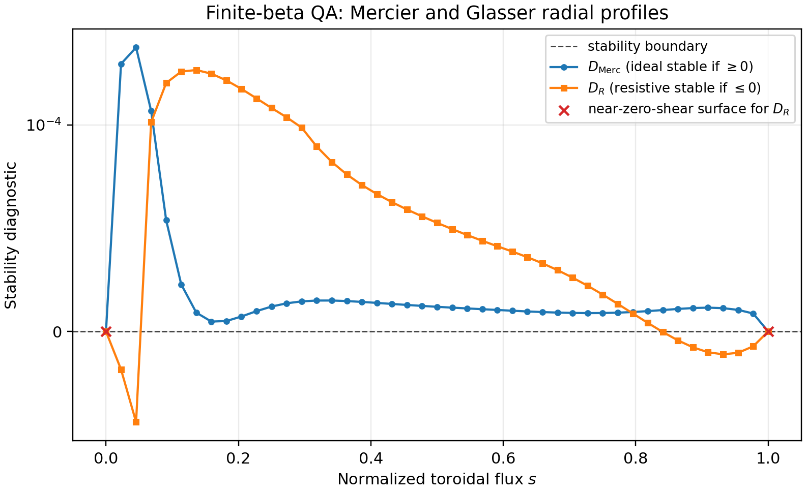
In this example, the finite-beta QA equilibrium is Mercier-stable on the
interior grid by D_Merc >= 0, while D_R becomes positive over part of
the radius. That behavior is expected: the Glasser correction is positive and
can make the resistive criterion more restrictive than the ideal Mercier gate.
Key VMEC2000 Convention: Parity Channels For bsubu/bsubv
VMEC2000 stores covariant components bsubu and bsubv in two “parity
channels” (the last dimension in Fortran is indexed 0:1). These channels
are not an even/odd-\(m\) decomposition of the physical field.
In the fixed-boundary output path, VMEC2000 forces IEQUI=1 before calling
funct3d and then computes (in bcovar.f) the odd-parity storage channel
as a scaled copy of the even channel:
where shalf is VMEC’s half-mesh \(\sqrt{s}\) factor (stored on the
full mesh index in the Fortran implementation but derived from the half mesh
radial locations).
Immediately upon entering jxbforce.f, VMEC2000 undoes this scaling before
performing its Fourier low-pass filter:
This means the two parity channels are primarily a storage/algorithmic convention: they let VMEC apply an \(m\)-dependent normalization rule inside its (mpol-1, ntor) filter loop without having to rebuild the parity split from Fourier coefficients.
What ``vmec_jax`` does
To match VMEC2000 output parity in the wout Mercier/jdotb diagnostics,
vmec_jax now constructs these parity channels the same way by default.
See: vmec_jax/wout.py (Mercier/jxbforce parity channel construction) and
VMEC2000 bcovar.f/jxbforce.f for the reference behavior.
JXBFORCE Low-Pass Filter (Conceptual Summary)
VMEC2000 applies a low-pass filter to the covariant components bsubu and
bsubv using a truncated set of modes:
poloidal: \(m \le \texttt{mpol}-1\)
toroidal: \(n \le \texttt{ntor}\)
The filtered fields are then used to compute cancellation-sensitive quantities
such as itheta, izeta, bdotk (and ultimately jdotb and Mercier
terms). The filter is implemented with VMEC’s precomputed trigonometric tables
(cosmui, sinmui, cosnv, sinnv, …) and includes VMEC’s Nyquist
half-weighting at the geometric Nyquist limits.
vmec_jax mirrors this by using the same VMEC trigonometric tables and the
same (mpol-1, ntor) cutoffs when building the wout diagnostics.
From Filtered Fields To jdotb (VMEC2000 Discretization)
After the filter, VMEC2000 reconstructs bsubsu and bsubsv and defines
two auxiliary fields (names follow the VMEC2000 source):
where \(h_s = 1/(ns-1)\) is the uniform VMEC radial grid spacing on the
normalized toroidal-flux grid and js is the (1-based) full-mesh radial
index.
Then:
with bsubu1/bsubv1 computed as VMEC’s half-mesh average
(\(\tfrac12(\cdot_{js+1}+\cdot_{js})\)).
Finally, VMEC2000 forms a 1D profile jdotb as a (weighted) flux-surface
average of bdotk with a volume normalization:
where \(\langle\cdot\rangle\) denotes a VMEC quadrature sum on the internal
(\(\theta,\zeta\)) grid and \(\sigma\) is the anisotropy factor
(sigma_an; \(\sigma\equiv 1\) for isotropic equilibria).
Numerical Sensitivity: Why jdotb Can Look Like Noise
For currentless / vacuum-like cases (e.g. inputs with effectively zero current
profile), the physically relevant signal in jdotb may be small. However,
VMEC2000’s discretization includes:
a radial finite difference amplified by \(1/h_s\),
cancellation-prone sums in the (mpol-1, ntor) Fourier low-pass filter,
axis and edge extrapolations, and
\(\sqrt{s}\)-weighted parity conventions.
As a result:
jdotbcan be dominated by discretization noise and cancellation error in some configurations,relative error comparisons become uninformative when the reference value is near zero or oscillatory, and
agreement should be evaluated in context (e.g. by checking that the full Mercier terms match and that
jdotbparity holds in cases where the signal is demonstrably nonzero).
In parity work we therefore adopt the VMEC community convention of excluding a small number of points near the magnetic axis and (optionally) the edge when comparing cancellation-limited stability diagnostics.
Profiles: QI_nfp2 + QA_lowres (jdotb should be small)
The following figures compare VMEC2000 vs vmec_jax profiles for two
configurations where jdotb is expected to be small and differences are not
physically meaningful. In both plots, we skip the first 6 radial points and
drop the edge point to avoid the most cancellation-limited region.
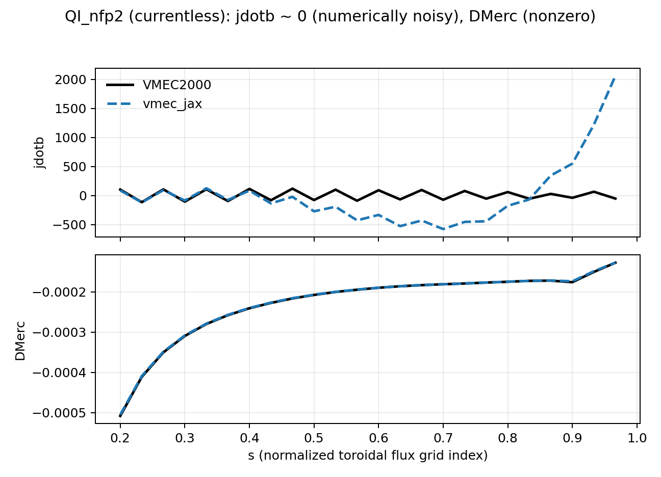
QI_nfp2: jdotb (cancellation-limited) and DMerc (nonzero).
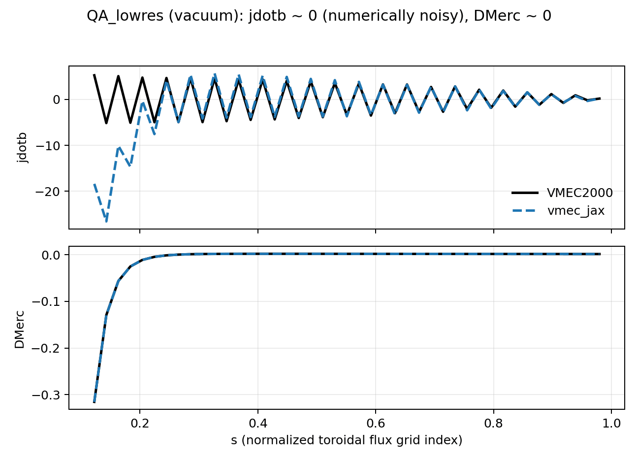
LandremanPaul2021_QA_lowres: vacuum-like case; DMerc should be ~0.
For current-driven cases, use the bundled reactor-scale QA/QH examples when a
nonzero jdotb profile is needed for targeted parity checks. The small-signal
QI/QA plots above remain the default documentation figures because they are the
most stable examples for explaining the cancellation-limited behavior of
jdotb and Mercier diagnostics.
Implementation Pointers (Source Code)
The relevant vmec_jax code paths are:
vmec_jax/wout.py:parity-channel construction for
bsub{u,v},jxbforce-style low-pass filter and reconstruction,
Mercier and
jdotbassembly.
Performance Notes (vmec_jax vs VMEC2000)
VMEC2000 implements these diagnostics in Fortran with explicit loops over
(m,n) modes and over the reduced (theta,zeta) grid. For parity work,
vmec_jax originally mirrored this ordering closely, including Python-level
loop nests for some cancellation-sensitive sums. That path is useful for
debugging, but it is too slow to be a good default.
Today, vmec_jax uses vectorized NumPy contractions (einsum) for the
wrout-style Nyquist analysis and the jxbforce filter by default. These
vectorized paths preserve the VMEC2000 discretization but may change floating
point summation order slightly.
If you need the slow loop order for debugging, the following env vars switch back to explicit loops:
VMEC_JAX_WROUT_LOOP=1: use loop-basedwroutNyquist analysis.VMEC_JAX_JXBFORCE_LOOP=1: use loop-basedjxbforcereconstruction ofbsubsu/bsubsv.VMEC_JAX_BSUB_FILTER_LOOP=1: use loop-basedjxbforcelow-pass filter.VMEC_JAX_MERCIER_EXACT_SUM=1: use explicittheta/zetasummation order in Mercier surface averages.
The reference VMEC2000 implementations are:
bcovar.f(odd-channel storage convention forIEQUI=1outputs)jxbforce.f(filter anditheta/izeta/bdotkconstruction)mercier.f(Mercier term assembly)
Reproducing The Figures
These figures were generated from VMEC-style wout_*.nc files using:
python tools/diagnostics/plot_wout_profiles_compare.py \
  --vmec /path/to/vmec2000/wout_case.nc \
  --jax  /path/to/vmec_jax/wout_case.nc \
  --vars jdotb,DMerc \
  --axis-skip 6 --drop-edge \
  --out docs/_static/figures/case_jdotb_dmerc_parity.png