Free-Boundary Coil Optimization

This page documents the research lane toward true single-stage free-boundary optimization with differentiable coils. The existing VMEC-compatible mgrid path remains the VMEC2000-compatibility backend; generated-mgrid WOUT parity is optional/non-promoted unless explicitly stated. The new direct-coil path evaluates the external field from coil Fourier coefficients and currents in JAX, so the coil parameters can become the independent optimization variables.

Architecture

The intended single-stage loop is:

coil Fourier dofs/currents
   -> differentiable Biot-Savart external field
   -> vmec_jax free-boundary equilibrium
   -> wout/proxy diagnostics
   -> coil-only objective update

Pedagogic forward examples

Two short examples in examples/ show the two free-boundary external-field paths without hiding the workflow inside a large sweep driver.

The compatibility path uses ESSOS coils to write a VMEC mgrid file, then runs vmec_jax using the same mgrid-style external-field backend used for VMEC2000 parity:

export ESSOS_ROOT=/Users/rogeriojorge/local/ESSOS_mgrid_pr
export ESSOS_INPUT_DIR=$ESSOS_ROOT/examples/input_files
PYTHONPATH=.:$ESSOS_ROOT:$PYTHONPATH \
  python examples/free_boundary_essos_mgrid_forward.py --max-iter 10

The direct-coil research path converts the same ESSOS coils to CoilFieldParams and passes them directly to run_free_boundary. No mgrid file is written or read by the solver:

export ESSOS_ROOT=/Users/rogeriojorge/local/ESSOS_mgrid_pr
export ESSOS_INPUT_DIR=$ESSOS_ROOT/examples/input_files
PYTHONPATH=.:$ESSOS_ROOT:$PYTHONPATH \
  python examples/free_boundary_essos_direct_forward.py --max-iter 10

Both examples accept --dry-run to write the input deck and JSON summary without running VMEC. This is useful for checking the generated namelist, magnetic-grid bounds, and direct-coil provider wiring. By default, outputs go under results/free_boundary_essos_mgrid_forward/ and results/free_boundary_essos_direct_forward/.

Boozer/QS diagnostics are the intended promotion target for this lane, but the current implementation keeps the single-stage optimization example on a cheap VMEC residual plus VMEC-state qs_total, aspect, and mean-iota proxy until complete Boozer/QS full-loop gradient checks pass.

Reviewer-facing validation plots for this lane are committed only as compressed summary panels. Generated WOUTs, magnetic grids, PDFs, and full-resolution raw renderings stay out of git. Use the reproduction commands below to regenerate the architecture, beta-scan, provider-parity, and benchmark figures from JSON summaries.

Phase 1 in this lane includes JAX-native coil-field sampling, an ESSOS coil adapter, generated-mgrid compatibility, and forward free-boundary solves from direct coils. Phase 2 targets the production custom adjoint through the full free-boundary vacuum/NESTOR solve. Several phase-2 validation rungs are already implemented on JAX-visible dense or accepted-state problems, but the production run_free_boundary nonlinear-loop adjoint is not claimed as publication-ready until complete-solve AD-vs-finite-difference checks pass. The current post-merge evidence now includes reusable accepted-trace replay helpers, accepted-state bsqvac replay derivatives with respect to the VMEC state, JAX-visible nonlinear-controller primitives with fixed-length masked lax.scan control flow, and a fixed-accepted-trace custom-VJP seam for direct-coil replay objectives. The fixed-trace path is guarded by accepted trace fingerprints so finite-difference promotions can reject perturbations that changed the adaptive host-controller branch. These validate the intended full-loop adjoint contract, but they are still production-adjacent validation gates rather than a promoted custom VJP for the host-controlled run_free_boundary loop.

Adjoint Validation Roadmap

The exact-gradient lane is deliberately staged. The literature points to a discrete-adjoint implementation around the structured spectral operators and linear solves, not to reverse-mode differentiation through every nonlinear iteration. In NESTOR, the free-boundary vacuum contribution is a spectral integral-equation solve for a Neumann problem on a toroidal surface; this naturally maps to a JAX-native operator plus an implicit transpose solve. JAX’s custom_linear_solve is the relevant primitive for this layer because it defines reverse-mode derivatives by solving the transposed linear problem at the converged solution rather than taping the internals of the linear solver. This is also consistent with recent spectral-PDE adjoint work, where efficient adjoints are built from reusable operator graphs, fast transforms, and sparse or structured linear solves.

The validation ladder is:

1. Provider derivatives: direct Biot-Savart derivatives with respect to coil current, Fourier curve coefficients, and evaluation coordinates.

2. Toy implicit vacuum chain: direct coils feed a dense custom-linear-solve vacuum problem, and gradients with respect to current and geometry are checked against finite differences.

3. Boundary projection: JAX vacuum-boundary projection derivatives with respect to sampled cylindrical fields and boundary coefficients.

4. Projected implicit vacuum chain: direct coils feed the JAX boundary projection and then a dense custom-linear-solve vacuum problem, with current and geometry gradients checked against finite differences.

5. Mode-space NESTOR chain: the same projected boundary data feeds dense_vmec_nestor_mode_solve_jax, a JAX-native VMEC-style operator that combines source symmetrization, mode-RHS projection, nonsingular Green-function source/matrix assembly, analytic/singular analyt.f source/matrix assembly, mode-matrix assembly, and dense mode-space solve that reconstructs the boundary scalar potential. This validates the differentiable operator blocks used by the VMEC-like NESTOR solve on low-resolution grids. The high-resolution matrix-free production operator remains phase-2 work.

6. Nonlinear fixed-point chain: direct-coil controls feed a dense nonlinear fixed-point solve with a custom implicit adjoint. The reusable direct_coil_projected_mode_fixed_point_jax helper implements the moving-boundary validation loop: the current state changes where the coil field is sampled, the field is projected through the JAX boundary projection and mode-space vacuum response, and the response updates the next state. The companion direct_coil_projected_mode_fixed_point_objective_jax helper wraps the solved state in a scalar quadratic objective with component diagnostics for optimizer-facing AD-vs-FD tests. The reusable pytree_directional_derivative_check_jax helper then compares exact pytree directional derivatives against central finite differences. The focused tests run that check on the scalar objective with respect to the full CoilFieldParams pytree, verifying finite, nonzero gradients and a mixed current/curve-coefficient directional derivative. This validates the mathematical reverse pass needed by the production free-boundary fixed-point wrapper: solve F_x^T lambda = dJ/dx at the accepted root and apply -F_p^T lambda to coil/current parameters. This is still a dense validation primitive, not the production VMEC nonlinear loop. The same phase-2 work now also includes a JAX-visible nonlinear-controller primitive: jax_visible_nonlinear_controller_jax and jax_visible_masked_nonlinear_controller_jax model a fixed-length differentiable controller with an on-device convergence mask. The tests check controller-level AD-vs-central-FD behavior for a direct-coil moving-boundary objective with current and Fourier geometry controls. This is the concrete replacement pattern for differentiating through convergence/early-stop logic without taping a Python host loop, but it is not wired in as the default production free-boundary controller yet. The accepted/rejected controller layer also includes jax_visible_segmented_accepted_nonlinear_controller_jax. This helper splits a long accepted-controller scan into static-policy subcontrollers, preserving the accepted state and convergence mask across segment boundaries. The unit gate compares the segmented run against the monolithic scan and checks the segmented objective gradient against both the monolithic gradient and a central finite difference. This is the validated structure needed for production traces that change radial preconditioner policy without padding every branch-local array into one large scan payload.

7. Full direct-coil free-boundary solve: low-resolution physical scalar objectives, first with one coil current and then with one Fourier coefficient, bounded against finite differences of complete solves. The promoted same-branch current representative includes a VMEC-state quasisymmetry-ratio scalar, qs_total, in addition to aspect ratio and accepted-vacuum scalars.

8. Boozer/QS objective: the same complete-solve finite-difference checks after Boozer/QS diagnostics are in the objective path.

The reviewer-facing status of this ladder is:

Rung	Status	Current validation evidence	Remaining promotion work
1	Complete	Coil Biot-Savart derivatives with respect to currents, Fourier curve coefficients, and evaluation coordinates are checked against finite differences.	None for the provider derivative layer.
2	Complete	Dense custom-linear-solve vacuum problems validate implicit gradients with respect to coil current and geometry controls.	None for the dense toy vacuum primitive.
3	Complete	Boundary-projection derivatives are checked with respect to sampled cylindrical fields and boundary coefficients.	None for the projection primitive.
4	Complete	Direct coils, boundary projection, and a dense implicit vacuum response are chained and AD-vs-FD checked for current and geometry controls.	None for this projected dense-chain primitive.
5	Complete for validation scale	dense_vmec_nestor_mode_solve_jax validates the JAX-visible VMEC-style source/RHS/matrix/mode-space blocks on low-resolution grids.	Replace the dense validation operator with the production matrix-free/high-resolution NESTOR adjoint.
6	Complete for validation scale	A dense nonlinear fixed-point loop validates the implicit-root reverse pass for current and Fourier-geometry controls. A JAX-visible masked nonlinear-controller primitive also validates the production replacement pattern for fixed-length scan control with early-stop masking.	Wrap or replace the production VMEC nonlinear free-boundary iteration with the same validated custom-adjoint contract.
7	Partial	Complete direct-coil solves have finite-difference response guards, and accepted-boundary replay has AD-vs-FD checks after freezing the accepted plasma boundary. Accepted-state bsqvac replay is also AD-vs-FD checked with respect to the VMEC boundary state. The fixed accepted-trace custom-VJP seam is now checked against complete-solve central finite differences on unchanged accepted branches for a current-only direction and for mixed current/Fourier-geometry directions.	The remaining production milestone is the general adaptive host-controller branch seam: accepted/rejected step selection, resets, activation cadence, and limiter branch changes remain unclaimed unless the explicit branch fingerprint is unchanged.
8	Open	The phase-1 coil-only optimization example currently uses a cheap VMEC residual plus VMEC-state qs_total, aspect, and mean-iota proxy instead of Boozer/QS gradients.	Add Boozer/QS diagnostics to the complete-solve objective and validate coil-current and coil-geometry gradients against finite differences.

In short, rungs 1–6 validate the mathematical and operator pieces needed for a production adjoint, rung 7 validates finite-response and accepted-state replay but not the host-controlled nonlinear iteration derivative, and rung 8 remains the publication-level coil-to-QS gradient target.

The first six AD-vs-FD rungs are implemented as fast tests today, and the fixed-boundary dense mode-space NESTOR rung is promoted for both stellarator-symmetric and LASYM tiny direct-coil cases: one coil current and one Fourier geometry coefficient are checked against central finite differences through the chain direct coils -> boundary projection -> VMEC/NESTOR source/matrix assembly -> dense mode solve while the plasma boundary is held fixed. The nonlinear fixed-point rung is also AD-vs-FD checked for a direct-coil current and one Fourier geometry coefficient, including a state-dependent boundary sample and projected mode-space vacuum response, but only on a dense validation loop solved inside JAX. The masked-controller rung then verifies that a fixed-length JAX scan with an on-device done mask keeps the final state and direct-coil gradients stable against finite differences. Rung 7 is split deliberately: complete accepted direct-coil solves have fast finite-difference response guards for current and one Fourier geometry coefficient. The same complete-solve guard now also evaluates the phase-1 coil-only proxy objective used by examples/optimization/free_boundary_QS_coil_optimization.py (VMEC residual plus aspect/iota terms) and checks finite central-difference responses to both coil controls. The accepted-state direct-coil normal-field metric also has a JAX replay gate whose current derivative matches central FD after freezing the accepted plasma boundary, and the accepted-state bsqvac replay path now matches central FD with respect to the packed VMEC state. The two-step accepted-trace replay path is also exposed through direct_coil_accepted_trace_directional_check_jax and checks current, Fourier-geometry, and mixed coil directions after resampling the second boundary from the first replayed accepted state. The full accepted-trace replay also preserves inactive/setup accepted steps and VMEC host-control reset discontinuities, such as the free-boundary turn-on reset, instead of incorrectly chaining every state_post into the next state_pre. The scalar direct_coil_fixed_trace_custom_vjp_objective_jax wrapper exposes this fixed accepted replay behind an explicit custom VJP. The newer direct_coil_accepted_trace_controller_custom_vjp_objective_jax wrapper uses the same frozen accepted steps but carries accepted/rejected masks, scalar update controls, velocity histories, and preconditioner arrays through the JAX-visible accepted-controller replay. This is the preferred phase-2 seam for production-adjacent validation. When production traces change the active radial preconditioner size across accepted steps, the controller replay keeps those preconditioner matrices branch-local instead of padding them into the scan payload; scalar controls and velocity histories remain scan-stacked. The reusable segmented accepted-controller primitive now validates the same split on a JAX-visible toy controller: segment boundaries are static Python structure, while each segment body is a differentiable lax.scan and the state/done carry is propagated across segments. Production replay has not yet been switched to this segmented primitive by default, but direct_coil_accepted_trace_controller_replay_objective_jax exposes an opt-in use_preconditioner_policy_segments mode that slices the stacked trace controls by the reported static-policy segments and validates identical accepted-output behavior against the monolithic replay. The production-backed test passes. Segment mode now builds local trace-switch branches for each static segment instead of recompiling a global switch over all accepted traces, but the current one-segment gate remains dominated by strict-update replay compilation, so the default stays monolithic until segmented replay compile cost is reduced on real multi-policy traces. direct_coil_accepted_trace_fingerprint_delta records whether a finite-difference perturbation stayed on the same accepted-step/control branch, including the same traced reset pattern, scalar update controls, preconditioner policy flags, active preconditioner size, and preconditioner/mode-shape signatures. The current required gate exercises this same-branch contract in three ways: a current-only perturbation validates the cleanest coil-control direction, a Fourier-coefficient-only perturbation validates a pure coil-geometry direction, and the existing stellsym/LASYM gate validates a mixed current plus Fourier-geometry direction. These tests compare the custom-VJP directional derivative to the central finite difference of complete tiny free-boundary solves after explicitly rejecting branch changes. This is stronger than a fixed-boundary replay test, but it remains a same-branch accepted-trace validation rather than a general derivative of the adaptive host loop. The current-only gate also promotes physical scalars from the same complete base/plus/minus solve triplet: final aspect ratio, VMEC-state quasisymmetry-ratio qs_total, accepted Bnormal RMS, and accepted Bsqvac RMS. The last two scalars exercise active free-boundary vacuum forcing seen by the accepted update, while still requiring identical accepted-trace and residual-controller fingerprints before comparing AD against central finite differences. The same current-only promotion now also replays one explicit fixed rejected controller slot with the accepted-only fast path disabled. This validates that the JAX-visible controller seam carries accepted/rejected masks and done controls through the custom-VJP scalar path instead of silently reducing the branch to accepted-only replay. This is still a fixed same-branch replay check; it does not claim derivatives through a host branch change that would alter which trial steps are accepted. For scripts that need reviewer-facing evidence, the companion direct_coil_accepted_trace_fingerprint_delta_summary helper converts the delta into a strict-JSON-safe payload. On the tiny forced-active default gate, the branch-compatible complete solve also compares both the fixed-trace custom-VJP directional derivative and the stacked-controller custom-VJP directional derivative against a central finite difference of the final accepted-state norm for a mixed coil current/Fourier direction, for both stellarator-symmetric and LASYM traces. This is the current promoted same-branch complete-solve validation, not yet a claim that arbitrary controller branch changes are differentiable.

The same evidence can be written as a local JSON artifact without adding generated data to the repository:

JAX_ENABLE_X64=1 python tools/diagnostics/direct_coil_same_branch_adjoint_report.py \
  --out /tmp/vmec_jax_freeb_same_branch_adjoint_report.json \
  --workdir /tmp/vmec_jax_freeb_same_branch_adjoint_report_work

The default command is bounded and records the branch fingerprints, complete-solve central finite-difference slope, and fixed-trace custom-VJP slope. The required CI gate is stricter than this default diagnostic: it also checks same-branch physical scalar slopes for aspect ratio, VMEC-state qs_total, and accepted Bnormal/Bsqvac RMS on the current-only representative. Passing --include-controller-vjp also evaluates the stacked accepted-controller custom VJP, which is useful for deeper review but slower in cold processes. The JSON report includes accepted_trace_controls.preconditioner_policy_segment_summary so reviewers can see whether the accepted trace is a single static preconditioner-policy range or will require multiple subcontrollers. The controller replay keeps only the tridiagonal preconditioner policy as branch-local static trace data. Update limiting and divide_by_scalxc_for_update are JAX-visible scan controls, so accepted controller payloads can include those switches without traced-Python-boolean failures. The fixed accepted replay is still well-defined because each accepted step is selected by a static lax.switch branch over the recorded trace index; the preconditioner policy is therefore fixed for that step and is covered by the same-branch fingerprint. The remaining controller refactor is to make the radial preconditioner policy itself JAX-visible, or to split the future production controller into static preconditioner-policy subcontrollers before claiming gradients through adaptive preconditioner-policy changes. The direct_coil_accepted_trace_preconditioner_policy_segments helper exposes the consecutive trace ranges with identical static preconditioner policy, precond_jmax, and preconditioner/mode payload shapes; this is the tested data model for that subcontroller split. The accepted-controller replay returns these ranges as preconditioner_policy_segments together with the segment count, so diagnostics can distinguish a same-policy replay from one that will need multiple static-policy subcontrollers before the replay implementation is refactored. The companion preconditioner_policy_segment_summary payload is JSON-safe and records the accepted, rejected, free-boundary replay, state-reset, and done-marker counts inside each static-policy range.

The segmented replay timing diagnostic is separate from the same-branch adjoint evidence:

JAX_ENABLE_X64=1 python tools/diagnostics/direct_coil_segmented_replay_report.py \
  --out /tmp/vmec_jax_freeb_segmented_replay_report.json \
  --workdir /tmp/vmec_jax_freeb_segmented_replay_work

By default this diagnostic synthesizes a two-policy accepted-trace sequence by flipping a static preconditioner policy flag on alternating traces while keeping trace payload shapes fixed. This exercises the segmented controller machinery and checks objective/final-state parity against the monolithic controller replay; it is not a claim that the synthetic policy sequence came from production. The current tiny local run passed with two segments, zero objective/state difference, and cold timings of about 7.59 s for the monolithic replay versus 7.56 s for segmented replay. That validates the control-flow split, but it does not yet demonstrate a meaningful speedup; the next performance target is a real multi-policy production trace or a larger trace-width benchmark. Running the same diagnostic on a slightly longer tiny solve without synthetic policy edits,

JAX_ENABLE_X64=1 python tools/diagnostics/direct_coil_segmented_replay_report.py \
  --out /tmp/vmec_jax_freeb_segmented_replay_nosynth_n4.json \
  --workdir /tmp/vmec_jax_freeb_segmented_replay_nosynth_n4_work \
  --niter 4 \
  --no-synthetic-multi-policy

produced a real two-segment accepted trace: the first step used precond_jmax=6 and the remaining three steps used precond_jmax=7 with active free-boundary replay. The segmented and monolithic replay objectives and final states matched exactly in the JSON report, but cold replay timing was still comparable: about 21.19 s monolithic versus 21.38 s segmented. This confirms the next optimization target is the strict-update and preconditioner replay compilation path itself, not just the controller segment wrapper. The same diagnostic also exposes an opt-in --segment-local-preconditioner-controls mode. This stacks preconditioner payloads independently inside each static-policy segment when global stacking is impossible. On the same four-step no-synthetic trace, both the default segmented replay and the segment-local variant preserved objective and final state exactly. The measured cold timings were still slightly slower than the monolithic path: about 21.01 s monolithic versus 21.80 s segmented without segment-local controls, and about 20.09 s monolithic versus 20.78 s segmented with segment-local controls. The option is therefore kept as a diagnostic hook, not as a promoted performance default. A narrower strict-update diagnostic isolates the accepted VMEC force, preconditioner, and update map by reusing stored freeb_bsqvac_half and excluding direct-coil boundary resampling:

JAX_ENABLE_X64=1 python tools/diagnostics/direct_coil_strict_update_replay_report.py \
  --out /tmp/vmec_jax_freeb_strict_update_replay_n4.json \
  --workdir /tmp/vmec_jax_freeb_strict_update_replay_n4_work \
  --niter 4

On the same tiny four-step setup, this isolated path passed with exact parity between trace-static controls and dynamic scalar/array/preconditioner controls. The first JIT call was about 0.446 s for trace-static controls and 0.536 s for dynamic controls, while warm calls were around 0.1 ms. This shows the standalone strict update is not the full ~21 s cold replay cost; the next performance rung should isolate boundary-geometry, direct-coil/NESTOR replay, and full-controller composition costs. A second isolation diagnostic times exactly that boundary-vacuum part:

JAX_ENABLE_X64=1 python tools/diagnostics/direct_coil_boundary_replay_report.py \
  --out /tmp/vmec_jax_freeb_boundary_replay_n4.json \
  --workdir /tmp/vmec_jax_freeb_boundary_replay_n4_work \
  --niter 4

On the same tiny active trace, fixed-geometry direct-coil/NESTOR replay took about 2.13 s for the first JIT call, while accepted-boundary geometry synthesis plus direct-coil/NESTOR replay took about 5.85 s. Both variants matched to ~9e-11 in objective value, and warm calls were below 0.3 ms. The remaining cold full-controller replay overhead is therefore controller composition across steps and repeated boundary replay compilation, not the standalone strict update. The remaining phase-2 blocker is differentiating through the nonlinear run_free_boundary iteration loop itself, rather than through the dense toy nonlinear primitive, fixed-boundary operator, complete finite-response proxy, or final fixed accepted-boundary replay. The combined JAX operator is also threaded into the free-boundary driver behind the opt-in VMEC_JAX_FREEB_JAX_NESTOR_OPERATOR=1 diagnostic flag for low-resolution validation. For stellarator-symmetric runs, the JAX path reconstructs the full VMEC angular grid internally for the nonsingular Green block while keeping the analytic/singular block on the active grid, matching the host bridge. The JAX operator closure can be precompiled and cached with VMEC_JAX_FREEB_JAX_NESTOR_JIT_OPERATOR=1 (the default when JIT is enabled), but the host bridge remains the production/default route because the compiled operator is still a validation primitive, not yet the final matrix-free adjoint. The production NESTOR adjoint is therefore still a phase-2 deliverable. The intended design is to expose a JAX-native NESTOR operator A(q) phi = b(q, I, c) where q is the VMEC boundary state and I, c are coil currents and curve coefficients. The backward pass should solve A(q)^T lambda = dJ/dphi and then use JAX JVP/VJP rules for the operator assembly and Biot-Savart source terms. This keeps memory independent of the number of vacuum-solver iterations and keeps gradient cost approximately independent of the number of coil optimization parameters.

Finite-pressure direct-coil support is currently a promoted forward validation lane: active NESTOR diagnostics respond to coil-current changes, matched direct/generated-mgrid provider samples agree tightly, and WOUT-level generated-mgrid/direct comparisons are bounded by the documented finite tolerances for the corrected ESSOS LP-QA stellarator pressure-continuation case. Accepted-equilibrium sensitivity and exact full-solve gradients remain phase-2 promotion gates.

Current Status

The current lane status is intentionally narrower than a production single-stage coil optimizer:

• mgrid remains the VMEC2000-compatible parity backend.

• Direct coils are supported as a JAX external-field provider for forward free-boundary solves, including nonzero pressure profiles.

• The finite-pressure evidence includes active-coupling provider validation and an LP-QA stellarator pressure-continuation lane. Generated-mgrid and direct-coil providers from the same ESSOS LP-QA coil set converge to actual WOUT beta values above 1%.

• The promoted high-resolution finite-beta reference evidence also includes the VMEC2000-compatible DIII-D mgrid benchmark: final ns=101, final FTOL=1e-12, and actual WOUT beta through 3.33%.

• The previous LP-QA direct-coil failure was traced to the automatic CPU lax.tridiagonal_solve preconditioner policy, not to direct Biot-Savart sampling or NESTOR bsqvac construction. The safe default now keeps the Thomas R/Z solve for direct free-boundary runs unless users force the lax path explicitly for diagnostics.

• The fast validation lane now includes same-branch complete-solve AD-vs-central-FD gates for direct-coil current, direct-coil Fourier geometry, and mixed stellsym/LASYM directions. These gates compare fixed accepted-trace/controller custom-VJP derivatives against complete-solve finite differences only after rejecting accepted-branch fingerprint changes.

• Branch-local production-forward replay gates now cover aspect ratio plus VMEC-state qs_total plus accepted Bnormal and Bsqvac RMS physical scalars, with scalar/vector coverage for current and Fourier geometry representatives. This validates a fixed accepted branch, not arbitrary adaptive host-controller branch changes.

• The phase-2 full-loop refactor target has JAX-visible masked and segmented nonlinear-controller primitives with AD-vs-FD direct-coil gradient coverage, plus accepted-state replay gates for coil and VMEC-state derivatives. This validates the replacement contract for the host loop but does not promote a default production run_free_boundary exact adjoint.

• The active NESTOR sensitivity checks validate the provider/coupling layer: normal-field/source channels scale linearly with current changes and bsqvac scales quadratically. They do not yet validate a full accepted equilibrium derivative.

• The phase-1 optimization example is coil-only, but it still uses a cheap VMEC residual plus VMEC-state qs_total, aspect, and mean-iota proxy. Boozer/QS objectives and production full-solve adjoints are next-step work.

• The experimental JAX NESTOR driver path is opt-in and guarded. It validates both LASYM full-grid and stellarator-symmetric reduced-grid samples, but the host bridge remains the default production path until complete-solve adjoints are promoted.

In short: direct-coil finite-pressure plumbing is present and validation-tested; high-resolution finite-beta mgrid validation exists for DIII-D; the LP-QA stellarator direct-coil forward lane has strict WOUT evidence through actual beta 1.93%; publication-grade gradients through the full free-boundary/NESTOR nonlinear loop and VMEC2000-bounded generated-mgrid trace parity are not claimed yet.

Low-Resolution Beta Scan

The first diagnostic uses unit-scale ESSOS Landreman-Paul QA coils and a pressure scan. The zero-pressure endpoint is retained as a reference, but the finite-pressure points are the meaningful provider-plumbing checks. The same coil set is used two ways:

1. ESSOS coils are sampled onto an mgrid file and solved by the legacy free-boundary compatibility path.

2. The same ESSOS coils are converted to CoilFieldParams and sampled directly by the differentiable JAX Biot-Savart provider.

The scalar diagnostics from the two vmec_jax providers agree within the recorded JSON precision/roundoff for this low-resolution validation run. The scan records both the input PRES_SCALE and the output energy ratio 100 W_p / W_B so future plots cannot accidentally validate only the vacuum case.

The default scan deliberately uses the unit-scale VMEC input examples/data/input.LandremanPaul2021_QA_lowres. Do not pair the default ESSOS LP-QA coils with the reactor-scale LP-QA input unless the coils are also scaled: the coil major radius is about 1.1 while the reactor-scale plasma has RBC(0,0) about 10.1. That mismatch was the cause of the failed high-res LP-QA run in the initial PR diagnostic.

The example uses --activate-fsq 1e99 by default. This forces immediate VMEC2000-style NESTOR turn-on so the short run exercises active finite-pressure vacuum coupling instead of stopping in the inactive ivac=-1 cadence. That is useful for provider validation. The residuals shown here are recomputed on the accepted final state with a fresh active NESTOR sample, but this is still not a converged high-beta result: the active residual norm remains large and must be bounded against VMEC2000 before this becomes a promoted finite-beta single-stage optimization claim.

Use --activate-fsq 1e-3 when checking literal VMEC2000 activation cadence. Use a larger value, such as the default 1e99, only when the goal is to force active coupling early in a deliberately short validation run. Those early-activation runs are provider/coupling diagnostics, not evidence that the accepted equilibrium is converged to the same state as a long VMEC2000 run.

The numerical summaries are runtime artifacts under the selected --outdir. They are intentionally not committed, since generated WOUT files, magnetic-grid files, and validation plots are handled as release/PR artifacts.

Reproduction

Run all commands in this section from the repository root. The ESSOS-backed commands require an ESSOS checkout on PYTHONPATH and the Landreman-Paul QA coil JSON under $ESSOS_INPUT_DIR. The beta-scan command exercises both the generated-mgrid and direct-coil backends; if your ESSOS checkout does not yet provide Coils.to_mgrid, add --skip-mgrid-runs to keep the direct-coil finite-beta scan runnable.

The three PR-review workflows are:

export ESSOS_ROOT=/path/to/ESSOS_mgrid_pr
export ESSOS_INPUT_DIR=$ESSOS_ROOT/examples/input_files

PYTHONPATH=.:$ESSOS_ROOT:$PYTHONPATH \
  python examples/free_boundary_essos_direct_forward.py \
  --input examples/data/input.LandremanPaul2021_QA_lowres \
  --max-iter 10 \
  --ns 7 \
  --mpol 3 \
  --ntor 2 \
  --nzeta 8 \
  --outdir results/free_boundary_essos_direct_forward

This ESSOS direct-coil forward run writes results/free_boundary_essos_direct_forward/input.lpqa_direct_coils, wout_direct_coils.nc, and summary.json. The summary records fsqr/fsqz/fsql, aspect, mean iota, coil length/current diagnostics, the DIRECT_COILS provider tag, mgrid: null, and the active free-boundary/NESTOR coupling diagnostics. Use the beta-scan command below when you need the standardized finite-beta pressure profile and the generated-mgrid comparison row.

The generated input deck contains MGRID_FILE='DIRECT_COILS' as a provider tag for the Python direct-coil examples. It is not a standalone magnetic-grid filename: replaying that generated input through the public vmec CLI alone will not reconstruct the ESSOS coils unless a direct-coil provider object is also supplied by Python. Use the example command above, or use the generated mgrid compatibility example when you need an input deck that can be replayed without Python coil parameters.

export ESSOS_ROOT=/path/to/ESSOS_mgrid_pr
export ESSOS_INPUT_DIR=$ESSOS_ROOT/examples/input_files

PYTHONPATH=.:$ESSOS_ROOT:$PYTHONPATH \
  python examples/free_boundary_essos_coils_beta_scan.py \
  --outdir results/free_boundary_essos_coils_beta_scan_smoke \
  --input examples/data/input.LandremanPaul2021_QA_lowres \
  --phiedge=-0.025 \
  --betas 0.0025 \
  --pressure-profile standard \
  --ns 12 \
  --max-iter 1000 \
  --ftol 1e-8 \
  --mpol 5 \
  --ntor 5 \
  --mgrid-nr 16 \
  --mgrid-nz 16 \
  --mgrid-nphi 16 \
  --activate-fsq 1e-3

This finite-beta scan writes summary.json plus wout_mgrid_beta_*.nc and wout_direct_beta_*.nc rows under the selected --outdir. When --skip-mgrid-runs is used, only the direct-coil WOUT rows are expected. The root summary is checkpointed after each case and contains complete, the coil/plasma scale summary, the mgrid path, the radial schedule, and per-run entries with backend, nominal beta label, WOUT path, residuals, aspect, mean iota, pressure, wp/wb beta proxy, and NESTOR history summaries. Staged scans additionally write case_checkpoints/*.json and per-stage WOUT/input files.

python examples/optimization/free_boundary_QS_coil_optimization.py \
  --smoke \
  --provider circle \
  --max-evals 1 \
  --max-iter 1 \
  --vmec-max-iter 2 \
  --helicity-m 1 \
  --helicity-n 0 \
  --qs-surfaces 0.25,0.5,0.75 \
  --pressure-profile standard \
  --beta 1.0 \
  --activate-fsq 1e99 \
  --outdir results/free_boundary_QS_coil_optimization_circle_smoke

This single-stage free-boundary coil-optimization smoke is dependency-light because it uses the synthetic circular direct-coil provider. It writes input.direct_coil_qs, history.json, summary.json, and wout_best_direct_coil_qs.nc. The optimizer vector contains only coil current and selected coil Fourier degrees of freedom; the plasma boundary is recomputed by the free-boundary solve at each objective evaluation. The current deterministic objective contains accepted-state VMEC residual, VMEC-state quasisymmetry-ratio residual, aspect-ratio, and mean-iota terms. The QS residual is evaluated from the accepted VMEC state, not from a promoted coil-to-Boozer exact adjoint through adaptive branch selection.

For a local same-branch validation artifact, add --write-same-branch-report. The default report mode is complete-solve finite-difference only and avoids the cold branch-local replay compilation. Use --same-branch-report-mode scalar to additionally validate one fixed-accepted-branch qs_total gradient, or vector to build the more expensive multi-scalar branch-local Jacobian for reviewer diagnostics. The scalar can be changed with --same-branch-report-scalar-key. Use aspect for a cheaper physical-scalar timing probe and qs_total for the QS-relevant scalar. The derivative report defaults to --same-branch-report-ad-mode direct, which differentiates the fixed accepted-branch replay directly and avoids an extra custom-VJP wrapper replay. Use --same-branch-report-ad-mode custom_vjp only when explicitly auditing the custom-VJP seam. The resulting same_branch_complete_solve_report.json includes a timings block. complete_solve_fd_wall_s measures the complete base/plus/minus finite-difference solves, while branch_local_scalar_wall_s or branch_local_vector_wall_s measures the fixed-accepted-branch replay derivative. On the current tiny circle-provider smoke, the forward objective evaluation is about two seconds, the complete finite-difference report is several seconds, and the first cold branch-local scalar replay can still take tens of seconds. That is why derivative-detail reports remain opt-in performance diagnostics rather than default example output. When scalar or vector detail is requested, the corresponding branch_local_* block also includes nested timing fields such as production_scalar_eval_wall_s, replay_value_and_grad_dispatch_s, replay_value_and_grad_ready_s, replay_vjp_wall_s, and replay_pullbacks_wall_s. These fields synchronize JAX arrays before recording device-ready timings, so they are suitable for distinguishing Python dispatch, XLA compilation, and CPU/GPU execution costs in local profiling.

Run the dependency-light direct-coil forward example from the repository root. This path constructs a synthetic circular CoilFieldParams object directly in vmec_jax and writes wout_direct_coils.nc plus summary.json without requiring ESSOS assets or an mgrid file.

python examples/free_boundary_direct_coils_forward.py \
  --max-iter 4 \
  --outdir results/free_boundary_direct_coils_forward

The direct-coil examples default to JIT force kernels, matching the public run_free_boundary fast path. Add --no-jit-forces only when debugging parity or compile behavior.

Run the ESSOS direct-coil forward example from the repository root. This path loads ESSOS coils, converts them to CoilFieldParams, runs one low-resolution finite-pressure free-boundary forward validation run without writing an mgrid file, and writes wout_direct_coils.nc plus summary.json.

export ESSOS_ROOT=/path/to/ESSOS_mgrid_pr
export ESSOS_INPUT_DIR=$ESSOS_ROOT/examples/input_files
PYTHONPATH=.:$ESSOS_ROOT:$PYTHONPATH \
  python examples/free_boundary_essos_direct_forward.py \
  --max-iter 10 \
  --outdir results/free_boundary_essos_direct_forward

Use --dry-run on the same command to validate the ESSOS coil conversion, the generated VMEC input deck, and the direct provider wiring without running VMEC. The generated input explicitly uses MGRID_FILE='DIRECT_COILS' and the JSON summary records mgrid: null. As above, DIRECT_COILS is a Python-provider tag, not a filesystem mgrid file.

Run the matched beta scan from the repository root. Until the ESSOS to_mgrid PR is merged and released, put the ESSOS branch checkout on PYTHONPATH. If only released ESSOS is available, add --skip-mgrid-runs to run the direct-coil provider without generating a magnetic grid.

export ESSOS_ROOT=/path/to/ESSOS_mgrid_pr
export ESSOS_INPUT_DIR=$ESSOS_ROOT/examples/input_files
PYTHONPATH=.:$ESSOS_ROOT:$PYTHONPATH \
  python examples/free_boundary_essos_coils_beta_scan.py \
  --outdir results/free_boundary_essos_coils_beta_scan_readme \
  --input examples/data/input.LandremanPaul2021_QA_lowres \
  --phiedge=-0.025 \
  --betas 0.00125 0.0025 0.00375 0.005 \
  --pressure-profile standard \
  --ns-array 16,31 \
  --niter-array 600,1200 \
  --ftol-array 1e-8,1e-8 \
  --mpol 5 \
  --ntor 5 \
  --mgrid-nphi 24 \
  --max-iter 1200 \
  --activate-fsq 1e-3

To include a self-consistent Redl bootstrap-current preconditioner before each finite-beta equilibrium solve, add:

--bootstrap-current-fixed-point \
--bootstrap-helicity-n 0 \
--bootstrap-max-fixed-point-iter 2 \
--bootstrap-n-current 32 \
--bootstrap-vmec-max-iter 1200 \
--bootstrap-ns-array 16,31 \
--bootstrap-niter-array 300,1200 \
--bootstrap-ftol-array 1e-7,1e-8 \
--bootstrap-damping 0.5 \
--bootstrap-max-current-update-norm 0.1 \
--bootstrap-return-best-evaluated-current

This leaves the plasma boundary and coils unchanged during the preconditioner; only the VMEC current profile is updated from the Redl formula. The scan summary records the per-case bootstrap-current history path, final CURTOR, effective damping, and current-step limiter status so these runs are auditable. The bootstrap-stage schedule controls are intentionally separate from the final scan NS_ARRAY/NITER_ARRAY/FTOL_ARRAY: use a cheaper Redl-current preconditioner schedule, then keep the final finite-beta equilibrium solve at the strict resolution required for validation. Treat the limiter as a continuation control: a coarse low-resolution Redl update can reduce the Redl mismatch while still worsening the next VMEC residual if the current step is too large. The best-evaluated-current option avoids handing the final beta solve a last proposed profile that has not yet been solved by the fixed-point loop.

Use staged radial continuation for high-resolution promotion attempts. Keep --pressure-continuation enabled so each pressure point starts from the previous accepted free-boundary LCFS. Add --resume-existing when rerunning an interrupted high-resolution scan: existing wout_{backend}_beta_*.nc files are skipped and, if their residuals satisfy --pressure-continuation-max-fsq, promoted as continuation seeds for the next pressure point. When --ns-array is supplied, the scan also writes case_checkpoints/{backend}_beta_*.json plus per-stage inputs and WOUT files after every accepted radial-grid stage. These stage checkpoints are independent of the root summary.json so a wall-time stop during a strict ns=51 or ns=101 stage still leaves the last accepted lower-resolution metrics and restart seed available to --resume-existing.

export ESSOS_ROOT=/path/to/ESSOS_mgrid_pr
export ESSOS_INPUT_DIR=$ESSOS_ROOT/examples/input_files
PYTHONPATH=.:$ESSOS_ROOT:$PYTHONPATH \
  python examples/free_boundary_essos_coils_beta_scan.py \
  --outdir results/free_boundary_essos_coils_beta_scan_highres_attempt \
  --input examples/data/input.LandremanPaul2021_QA_lowres \
  --phiedge=-0.025 \
  --betas 0 0.5 1.0 1.25 \
  --pressure-profile standard \
  --pressure-continuation \
  --resume-existing \
  --pressure-continuation-max-fsq 1e-6 \
  --ns-array 16,31,51,101 \
  --niter-array 1000,2000,4000,12000 \
  --ftol-array 1e-8,1e-10,1e-11,1e-12 \
  --mpol 5 \
  --ntor 5 \
  --activate-fsq 1.0

The --betas values are nominal pressure-scaling labels used to drive the scan. The actual physical beta must be read from summary.json or the WOUT file after convergence.

High-Resolution DIII-D Finite-Beta Benchmark

The current reviewer-facing high-resolution axisymmetric finite-beta evidence is the VMEC2000-compatible DIII-D mgrid benchmark.

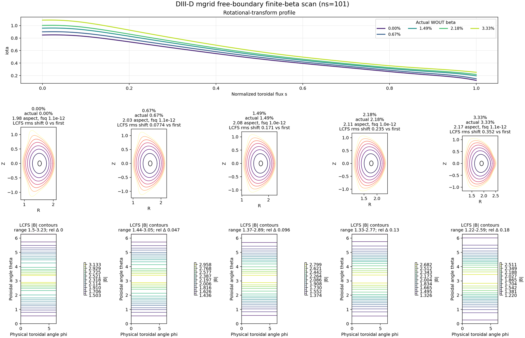
DIII-D mgrid free-boundary finite-beta scan at final ns=101 and FTOL=1e-12. The compressed figure is committed for PR review; the numerical summary is available as CSV.

Full-resolution external artifacts remain available for review without committing large vector/PDF files:

• WOUT-panel SVG: https://gist.githubusercontent.com/rogeriojorge/f9bfe56c5de71445cf86ea0843dc6629/raw/diiid_mgrid_beta_ns101_panel.svg

• WOUT-panel CSV: https://gist.githubusercontent.com/rogeriojorge/f9bfe56c5de71445cf86ea0843dc6629/raw/diiid_mgrid_beta_ns101_panel_summary.csv

The plotted WOUTs use final ns=101 and final FTOL=1e-12. The actual WOUT beta values shown in the compressed panel are 0.00%, 0.67%, 1.49%, 2.18%, and 3.33%; all final residual sums are near 1e-12. The renderer annotates LCFS RMS displacement and relative LCFS |B| RMS change against the vacuum row. At actual WOUT beta 3.33%, the LCFS RMS displacement is about 0.352, the maximum LCFS displacement is about 0.478, the magnetic-axis R-shift is about 0.381, and the relative LCFS |B| RMS change is about 0.181. This is promoted as a free-boundary finite-beta mgrid validation artifact. It is not a direct-coil stellarator promotion artifact.

For this DIII-D mgrid row only, executable-backed VMEC2000 validation was run on the same 3.33% WOUT row. The VMEC2000 and vmec_jax high-beta WOUTs agree far below the finite-beta response: aspect differs by 6.4e-7, rmnc relative RMS by 5.6e-7, zmns relative RMS by 3.5e-7, bmnc relative RMS by 5.1e-7, and LCFS RMS displacement between codes by 1.7e-6. The beta-induced LCFS RMS shift is therefore about five orders of magnitude larger than the vmec_jax-vs-VMEC2000 geometric mismatch.

Generate the DIII-D WOUTs from the bundled input and fetched mgrid asset:

python tools/fetch_assets.py --bundle reference-nc
python tools/diagnostics/run_diiid_mgrid_beta_scan.py \
  --outdir results/freeb_diiid_mgrid_beta_ns101 \
  --pressure-scales 0 0.50 1.0 1.35 1.8 \
  --ns-array 16,51,101 \
  --niter-array 1000,4000,20000 \
  --ftol-array 1e-8,1e-11,1e-12

Then render the panel directly from the generated summary:

python tools/diagnostics/render_freeb_beta_wout_panels.py \
  --summary results/freeb_diiid_mgrid_beta_ns101/summary.json \
  --title "DIII-D mgrid free-boundary finite-beta scan (ns=101)" \
  --stem diiid_mgrid_beta_ns101_panel \
  --outdir /tmp/freeb_publication_panels

High-Resolution LP-QA Stellarator Gate

The corrected unit-scale LP-QA input and ESSOS coil pair has two validation layers. The strict direct-coil ns=101 WOUT panel is phase-1 promoted forward-validation stellarator evidence. The lower-resolution ns=16,31 rows below are provenance and pressure-continuation diagnostics that explain how the basin was reached; they are not the publication-grade promotion rows. A local ns=16,31 run with PHIEDGE=-0.025 and PRES_SCALE = 1000 * nominal_beta_percent produced:

Nominal beta label	Actual WOUT beta	WOUT fsqr+fsqz+fsql	Aspect	Mean iota
0.0	0.00%	1.66e-8	6.013	0.409
0.5	0.72%	1.67e-8	6.046	0.405
1.0	1.49%	1.02e-8	6.098	0.395
2.0	3.43%	7.94e-7	6.343	0.191

The same low-resolution pressure-continuation schedule also follows the direct differentiable coil provider after disabling the unsafe automatic CPU lax.tridiagonal_solve R/Z preconditioner policy:

Nominal beta label	Actual WOUT beta	WOUT fsqr+fsqz+fsql	Aspect	Mean iota
0.0	0.00%	1.63e-8	6.014	0.405
0.5	0.72%	1.73e-8	6.048	0.402
1.0	1.49%	1.80e-8	6.097	0.393
2.0	3.42%	4.74e-7	6.343	0.201

These low-resolution rows are not the promoted phase-1 claim; the strict ns=101 WOUT panel below is. Neither row set promotes the full nonlinear exact-adjoint path: current gradient validation still stops at accepted-boundary replay and dense low-grid NESTOR primitives.

Lessons from the earlier failed attempts:

• pairing the default ESSOS coils with the reactor-scale LP-QA input is invalid without coil scaling and caused the original high-resolution failure;

• the native reactor-scale PHIEDGE has the wrong sign for the vacuum subroutine, while a small hand-tuned flux magnitude destroys the scale;

• direct pressure jumps are much less robust than pressure continuation from accepted lower-beta equilibria;

• the direct provider needs the safe Thomas R/Z preconditioner by default. Forcing the CPU lax tridiagonal path can generate a nonphysical first active R/Z update even when direct and generated-mgrid bsqvac agree to roughly 1e-3 relative RMS.

The promoted strict direct-coil ns=101 local continuation run converged the vacuum, nominal 0.5, nominal 1.0, and refined nominal 1.25 beta labels at final FTOL=1e-12. The corresponding actual WOUT beta values are 0.00%, 0.724%, 1.508%, and 1.932% with residual sums below 6.3e-12. A nominal 2.0 label reaches actual WOUT beta about 3.184% and residual sum 3.75e-7 from the same continuation sequence; that row is useful stress evidence but is not part of the strict promoted panel. This is committed PR-review artifact evidence, not a default CI gate and not a VMEC2000 generated-mgrid WOUT parity promotion.

The strict direct-coil LP-QA reviewer WOUT-panel is committed as a compressed summary figure:

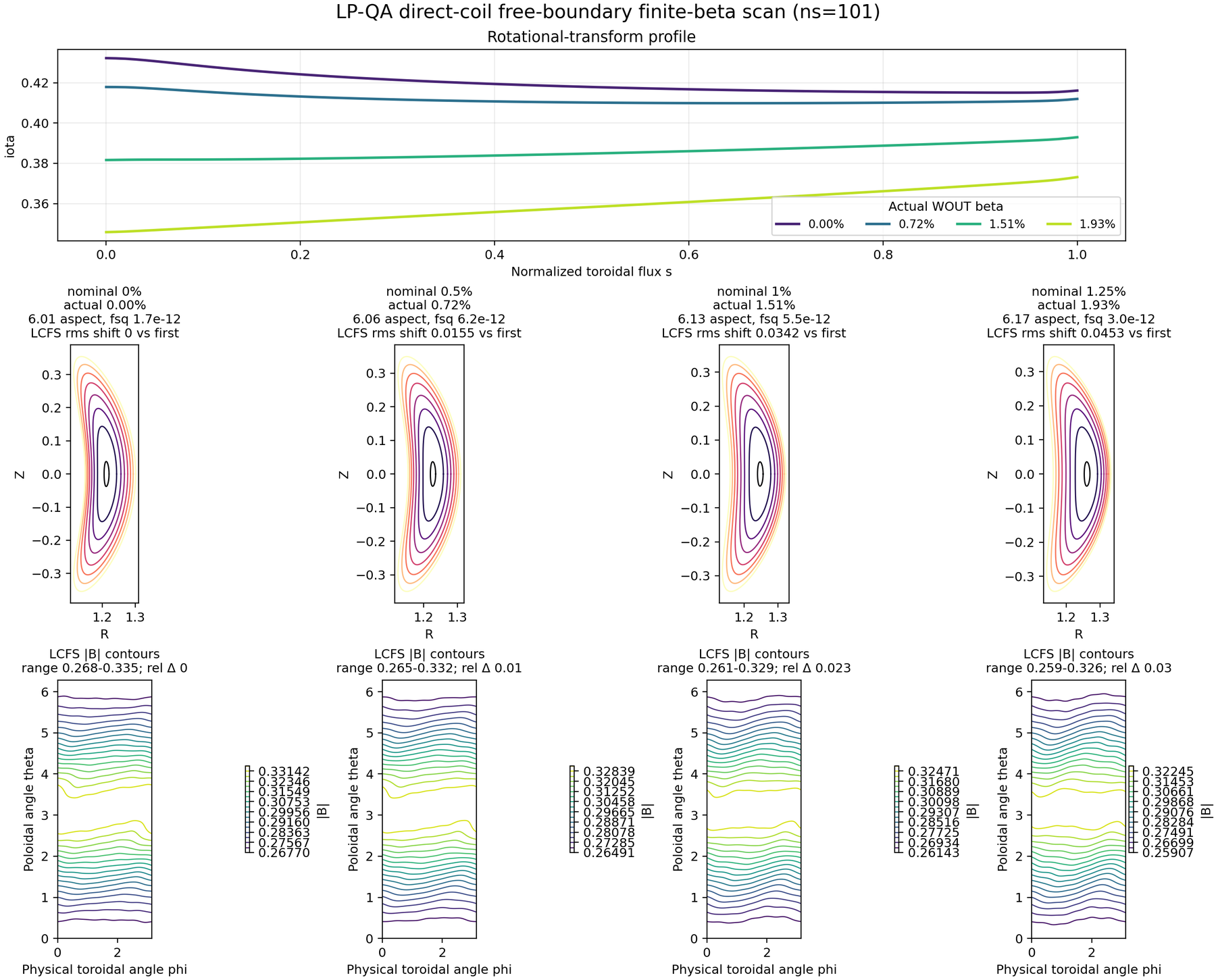
LP-QA direct-coil free-boundary finite-beta scan at final ns=101. The strict promoted rows reach actual WOUT beta through 1.932% with residual sums below 6.3e-12. The numerical summary is available as CSV.

Full-resolution external artifacts remain available for review:

• WOUT-panel SVG: https://gist.githubusercontent.com/rogeriojorge/f9bfe56c5de71445cf86ea0843dc6629/raw/lpqa_direct_coil_beta_ns101_panel.svg

• WOUT-panel CSV: https://gist.githubusercontent.com/rogeriojorge/f9bfe56c5de71445cf86ea0843dc6629/raw/lpqa_direct_coil_beta_ns101_panel_summary.csv

The WOUT-panel renderer is reusable for both mgrid and direct-coil scans:

The strict LP-QA panel was generated by first running the high-resolution pressure-continuation command above for nominal labels 0, 0.5, 1.0, and the refined 1.25 point. If the scan was interrupted, rerun the same command with --resume-existing so each accepted WOUT is reused as the next pressure-continuation seed.

python tools/diagnostics/render_freeb_beta_wout_panels.py \
  --summary results/free_boundary_essos_coils_beta_scan_highres_attempt/summary.json \
  --backend direct \
  --max-actual-beta 2.05 \
  --title "LP-QA direct-coil free-boundary finite-beta scan (ns=101)" \
  --stem lpqa_direct_coil_beta_ns101_panel \
  --outdir /tmp/freeb_publication_panels

For ad hoc existing DIII-D WOUTs, the renderer also accepts explicit files:

python tools/diagnostics/render_freeb_beta_wout_panels.py \
  --wout "0.00%=wout_diiid_b0_mg101.nc" \
  --wout "0.67%=wout_diiid_b050_mg101.nc" \
  --wout "1.49%=wout_diiid_b100_mg101.nc" \
  --wout "2.18%=wout_diiid_b135_mg101.nc" \
  --wout "3.33%=wout_diiid_b180_mg101.nc" \
  --title "DIII-D mgrid free-boundary finite-beta scan (ns=101)" \
  --stem diiid_mgrid_beta_ns101_panel \
  --outdir /tmp/freeb_publication_panels

Direct-provider nonlinear-control diagnostics now record accepted NESTOR histories for bnormal, gsource, bsqvac, and source reuse. A short LP-QA vacuum trace showed that the unsafe lax tridiagonal path converted identical raw R/Z residual blocks into an oversized first active update. The public driver still exposes limit_update_rms and the beta-scan example exposes --direct-coil-limit-update-rms for future nonlinear-control diagnostics, but the LP-QA promotion result above does not require that limiter.

Generate the benchmark summary used by the README/docs figure renderer:

python tools/benchmarks/bench_freeb_direct_coil_matrix.py \
  --quick \
  --out results/bench_freeb_direct_coil_matrix/summary.json

Render the README/docs figures from the generated JSON summaries:

python tools/diagnostics/render_freeb_single_stage_readme.py \
  --summary results/free_boundary_essos_coils_beta_scan_readme/summary.json \
  --benchmark-summary results/bench_freeb_direct_coil_matrix/summary.json \
  --outdir docs/_static/figures

The example writes input.* decks, wout_*.nc files, a generated mgrid, and summary.json in the output directory. Those runtime files are ignored by git; the committed figures and CSV are generated artifacts for documentation only.

Single-Stage Coil-Only Optimization Validation

The initial single-stage optimization example is a bounded validation example. It optimizes only coil currents and selected coil Fourier coefficients. The VMEC plasma boundary coefficients are never included in the optimization vector; the plasma surface is recomputed by a direct-coil free-boundary solve at every objective evaluation.

The default deterministic objective is:

• accepted-state VMEC residual,

• VMEC-state quasisymmetry-ratio residual,

• aspect-ratio target,

• mean-iota target.

The example records history.json, summary.json, and the best wout. It exits with code 77 when optional ESSOS assets are unavailable. For a dependency-light setup check that does not run VMEC or the optimizer, use --dry-run. This writes summary.json with the generated VMEC input path, selected coil variables, objective weights, QS helicity/surface settings, and baseline coil diagnostics. The summary also carries a single_stage_limitations list so dry-run artifacts remain self-describing when shared without this page:

python examples/optimization/free_boundary_QS_coil_optimization.py \
  --smoke \
  --dry-run \
  --provider circle \
  --helicity-m 1 \
  --helicity-n 0 \
  --outdir results/free_boundary_QS_coil_optimization_circle_preview

The same dry-run contract is covered for the optional ESSOS provider in CI by monkeypatching a synthetic ESSOS coil provider. The generated VMEC deck uses MGRID_FILE='DIRECT_COILS' and no generated mgrid artifact, so the example remains a direct-coil path:

export ESSOS_ROOT=/path/to/ESSOS_mgrid_pr
export ESSOS_INPUT_DIR=$ESSOS_ROOT/examples/input_files
PYTHONPATH=.:$ESSOS_ROOT:$PYTHONPATH \
  python examples/optimization/free_boundary_QS_coil_optimization.py \
  --smoke \
  --dry-run \
  --provider essos \
  --helicity-m 1 \
  --helicity-n 0 \
  --outdir results/free_boundary_QS_coil_optimization_essos_preview

For a bounded validation run, use the synthetic circular coil provider:

python examples/optimization/free_boundary_QS_coil_optimization.py \
  --smoke \
  --provider circle \
  --max-evals 1 \
  --max-iter 1 \
  --vmec-max-iter 2 \
  --helicity-m 1 \
  --helicity-n 0 \
  --qs-surfaces 0.25,0.5,0.75 \
  --pressure-profile standard \
  --beta 1.0 \
  --activate-fsq 1e99 \
  --outdir results/free_boundary_QS_coil_optimization_circle_smoke

For the ESSOS Landreman-Paul QA coils, put ESSOS on PYTHONPATH and use:

export ESSOS_ROOT=/path/to/ESSOS_mgrid_pr
export ESSOS_INPUT_DIR=$ESSOS_ROOT/examples/input_files
PYTHONPATH=.:$ESSOS_ROOT:$PYTHONPATH \
  python examples/optimization/free_boundary_QS_coil_optimization.py \
  --smoke \
  --max-evals 3 \
  --helicity-m 1 \
  --helicity-n 0 \
  --outdir results/free_boundary_QS_coil_optimization_essos_smoke

The promoted complete-loop gate now covers a VMEC-state qs_total scalar on the same fixed accepted branch as the aspect and accepted-vacuum scalars. The next scientific promotion step is replacing that VMEC-state proxy in this example with a Boozer-space QS objective and validating the same complete-loop gradients through the full Boozer/QS diagnostic path. The adaptive host branch selection itself remains outside the promoted derivative claim.

Each accepted objective evaluation records a weighted objective-term breakdown for the residual, QS, aspect-ratio, and mean-iota terms.

Benchmarks

This lane includes lightweight, non-CI benchmark scripts. The recommended first command is the matrix runner:

python tools/benchmarks/bench_freeb_direct_coil_matrix.py \
  --quick \
  --out results/bench_freeb_direct_coil_matrix/summary.json

The matrix runner executes the provider, direct free-boundary solve with and without JIT force kernels, and coil-gradient scripts with small CPU-only defaults. It writes each child JSON into the output directory and records the child paths plus compact timing/status rows in summary.json. GPU rows are opt-in:

python tools/benchmarks/bench_freeb_direct_coil_matrix.py \
  --quick \
  --include-gpu \
  --backend-note "local workstation validation" \
  --out results/bench_freeb_direct_coil_matrix_gpu/summary.json

If no JAX GPU device is available, the matrix records a skipped GPU row rather than falling back silently to CPU. Use --no-quick only for a larger local benchmark budget.

The benchmark CSV/JSON is written to the requested results directory. The runner probes concrete accelerator platforms, so mixed launches such as JAX_PLATFORMS=cpu,cuda still record CUDA rows even when CPU is the default backend. The current office benchmark shows tiny direct free-boundary solves are CPU-favorable, while provider and gradient microbenchmarks have small enough kernel payloads that CUDA launch overhead dominates. GPU production work should therefore focus on larger batched/tangent workloads and accepted-point replay amortization, not on claiming a speedup from these tiny validation cases.

The matrix keeps two direct-solve rows: the non-JIT diagnostic path and the default fast path with --jit-forces. On the 2026-05-25 office CUDA probe, --jit-forces reduced the tiny GPU warm direct solve from roughly 2.07 s to 0.31 s by removing the force-evaluation bucket as the dominant cost. The follow-up free-boundary-aware fused strict update then reduced the tiny CUDA warm solve further to about 0.25 s by cutting the update-state bucket to about one millisecond. The remaining warm GPU overhead is dominated by host-side iteration-control dispatch between preconditioning and accepted updates, while final NESTOR sample/solve time is already small. A split control-timing probe then localized that overhead to iteration_control_badjac_s, the early bad-Jacobian state check. The default keeps the first-two-iteration VMEC safety probe; use VMEC_JAX_BADJAC_INITIAL_STATE_PROBE_ITERS=0 only as an explicit profiling knob while checking VMEC2000 parity. On the tiny active direct-coil CUDA probe, that opt-in path reduced warm time from 0.269 s to 0.184 s and reduced the bad-Jacobian control bucket from 77 ms to below 1 ms.

The 2026-05-28 office CPU/CUDA rerun with concrete-platform GPU probing showed the same conclusion with finer buckets. The best --jit-forces tiny direct-solve row was 0.0525 s warm on CPU and 0.2346 s warm on CUDA. The force kernel itself was already competitive on CUDA (0.00855 s CUDA versus 0.00921 s CPU), and final NESTOR sample/solve time was also comparable. The remaining CUDA overhead was setup (0.0538 s versus 0.00931 s), residual scalar materialization (0.0293 s versus 0.000764 s), accepted-control fsq1 (0.0142 s versus 0.000146 s), and preconditioner dispatch (0.0126 s versus 0.00109 s). The next GPU patch should therefore cache or stage static setup and reduce scalar/control dispatch; scalar-defer is not yet the right default because those residual scalars still drive VMEC control flow and output history.

At the same head, the solver also uses a host flux-profile fast path for concrete default-APHI iota profiles. This is a safe setup-only optimization for non-traced forward solves; differentiated/traced profile coefficients still use the JAX path. The follow-up office matrix reported the same performance conclusion: the tiny direct-coil --jit-forces row was 0.0521 s warm on CPU and 0.2318 s warm on CUDA, while force assembly itself was still near parity. The remaining work is setup/control staging, not Biot-Savart kernel math.

The host-profile setup path is controlled by VMEC_JAX_HOST_PROFILE_SETUP. With the default auto policy, the latest office CUDA matrix keeps host fsq1 norms enabled but leaves primary residual products on device. The direct-coil JIT-forces row measured 0.224 s warm on CUDA with the old host-residual policy and 0.181 s when residual products were kept on device. The matrix also tested VMEC_JAX_TRIDI_PRECOMPUTE=1 and VMEC_JAX_TRIDI_SOLVE=1; both were slower than the default on the tiny direct-coil GPU row. Preconditioner dispatch/application and cold accepted-point force setup remain the next production GPU targets.

The same benchmark pass tested existing opt-in knobs and did not promote them: VMEC_JAX_HOST_UPDATE_ON_ACCELERATOR=1 was slower for the tiny CUDA row, and VMEC_JAX_BADJAC_INITIAL_STATE_PROBE_ITERS=0 was not a robust speedup after the current accepted-control fusion. Timing-light rows confirmed that timing instrumentation is not the dominant remaining wall-time source.

The June 2026 follow-up matrix kept the same conclusion. The production jit_forces=True row remains the large win: on the tiny direct-coil free-boundary case the no-JIT CUDA warm solve was about 13.3x slower than CPU, while the JIT-force row reduced that to about 2.7x. Host-policy ablations did not beat the production JIT row on CPU or CUDA, so they remain diagnostic controls. Quiet performance-mode direct-provider free-boundary runs now enable light_history by default, which suppresses broad per-iteration histories without changing the solver branch, NESTOR coupling, or convergence logic. The next real performance seam remains first-call force/tape construction plus GPU preconditioner/setup/finalize launch overhead.

The direct-solve child JSON includes active and trial NESTOR timing summaries: sample time, scalar-potential solve time, reuse counts, failed trial counts, and the final recompute sampler/solver timings. It also records a final_recompute_guard block for direct-solve children. This block compares the final accepted-state residuals against the pre-update final residuals, records final-vacuum metric deltas, and keeps safe_to_skip_final_recompute false until an explicit cached-finalization path proves parity. The matrix runner also enables VMEC_JAX_TIMING=1 and VMEC_JAX_TIMING_DETAIL=1 for the direct-solve child and records compact cold/warm solve-loop buckets in summary.json: force evaluation, preconditioner, update, trace construction, and unattributed iteration-loop cost. These fields are the first place to inspect when a direct-coil free-boundary solve is slow, because they separate Biot-Savart sampling, the vacuum linear solve, solver-trial replay overhead, and the higher VMEC residual/update loop. The setup bucket is also split into static-grid rebuild, free-boundary policy, boundary/profile construction, cache-key hashing, ptau constants, mode-index constants, and update constants, so GPU setup work can be targeted without conflating it with the NESTOR solve.

The child scripts are still useful when isolating one lane:

python tools/benchmarks/bench_external_field_providers.py \
  --points 48 --segments 48 \
  --out results/bench_external_field_providers.json

python tools/benchmarks/bench_freeb_direct_coil_solve.py \
  --max-iter 2 \
  --out results/bench_freeb_direct_coil_solve.json

python tools/benchmarks/bench_freeb_coil_gradient.py \
  --points 24 --segments 48 --matrix-size 24 \
  --out results/bench_freeb_coil_gradient.json

Each benchmark writes JSON with backend/device information, cold/compile timing, warm timing, and the problem dimensions. Defaults are intentionally small and CPU-safe; GPU production benchmarks should raise the grid and segment counts explicitly.

Optional VMEC2000 Diagnostics

The direct-coil provider is a vmec_jax research path; VMEC2000 itself reads external fields through mgrid files, not CoilFieldParams. VMEC2000 diagnostics therefore validate the generated-mgrid/free-boundary operator side of the branch, while direct-coil evidence comes from direct-versus-generated-mgrid comparisons inside vmec_jax.

The standalone three-way diagnostic writes a JSON report for the current research case. It always compares vmec_jax generated-mgrid against vmec_jax direct coils, then attempts VMEC2000 generated-mgrid if the executable is available. The generated mgrid is an interpolated compatibility backend, while direct coils sample the continuous Biot-Savart field. For one-update or short bounded traces this is a strict provider regression check. For longer active nonlinear free-boundary traces it is a finite-resolution convergence diagnostic: the accepted surface must remain inside the generated-mgrid box, residuals must be physical, and the direct/generated differences should decrease as the grid is refined.

export ESSOS_ROOT=/path/to/ESSOS_mgrid_pr
export ESSOS_INPUT_DIR=$ESSOS_ROOT/examples/input_files
PYTHONPATH=.:$ESSOS_ROOT:$PYTHONPATH \
  python tools/diagnostics/compare_freeb_coils_mgrid_vmec2000.py \
    --out results/freeb_coils_mgrid_vmec2000.json \
    --workdir results/freeb_coils_mgrid_vmec2000_work \
    --ns-array 5,9,13 \
    --niter-array 100,500,2000 \
    --ftol-array 1e-8,1e-10,1e-12

For a quick provider-only validation run, skip VMEC2000 explicitly:

export ESSOS_ROOT=/path/to/ESSOS_mgrid_pr
export ESSOS_INPUT_DIR=$ESSOS_ROOT/examples/input_files
PYTHONPATH=.:$ESSOS_ROOT:$PYTHONPATH \
  python tools/diagnostics/compare_freeb_coils_mgrid_vmec2000.py \
    --niter 1 \
    --mgrid-nphi 4 \
    --skip-vmec2000 \
    --activate-fsq 1e99 \
    --out results/freeb_coils_mgrid_vmec2000_smoke.json

The diagnostic defaults NZETA to --mgrid-nphi so the generated mgrid toroidal grid is compatible with VMEC’s free-boundary loader. If you override --nzeta, choose a value compatible with the generated grid (kp). Use --activate-fsq 1e99 only for short parity diagnostics so vmec_jax exercises the active NESTOR/free-boundary coupling immediately instead of proving only inactive-cadence bookkeeping. Do not use forced activation as long-trace promotion evidence unless the resulting surfaces stay inside the generated-mgrid domain and the final residuals are small. The JSON records active_free_boundary for both the direct-coil and generated-mgrid vmec_jax backends, approximate LCFS boundary_extents for each WOUT, and comparisons.vmec_jax_direct_vs_generated_mgrid.boundary_vs_mgrid_domain. That containment block reports whether each final surface is inside the generated grid and gives signed margins to the radial and vertical domain limits. The default direct/generated comparison tolerances are --jax-rtol 1e-5 and --jax-atol 1e-7; stricter values can be used for one-update provider regressions, while resolved free-boundary traces should be judged by mgrid-resolution convergence. When a generated mgrid has more toroidal planes than VMEC NZETA, vmec_jax follows VMEC2000’s read_mgrid_nc reduction and samples file planes 0, nskip, 2*nskip, ... instead of taking the first NZETA planes.

A bounded LP-QA low-resolution check illustrates the promoted interpretation. With examples/data/input.LandremanPaul2021_QA_lowres, ns=12, niter=300, default activation cadence, mgrid=24x24x8, and pressure-scale=1000, both vmec_jax backends enter active free-boundary coupling, stay inside the generated grid, and converge to fsq_total≈6e-4. Refining the generated grid to 48x48x16 reduces the direct/generated aspect relative gap to about 1.3e-4 and the iota-profile relative RMS to about 3.5e-3. This is finite-resolution evidence for the continuous direct-coil provider, not a claim that a coarse generated mgrid and direct Biot-Savart sampling are bitwise equivalent.

The forced-active reactor-scale LP-QA stress test is intentionally retained as a failure-mode diagnostic. In that run the nonlinear direct/generated surfaces leave the generated grid and cross into nonphysical R<=0 geometry, so generated-mgrid interpolation clips while the direct provider continues sampling a non-toroidal surface. The comparator now reports this explicitly with vmec_jax_*_boundary_outside_generated_mgrid warnings rather than allowing the result to be mistaken for provider-parity evidence.

To reproduce the bounded low-resolution finite-resolution probe:

export ESSOS_ROOT=/path/to/ESSOS_mgrid_pr
PYTHONPATH=.:$ESSOS_ROOT:$PYTHONPATH JAX_ENABLE_X64=1 \
  python tools/diagnostics/compare_freeb_coils_mgrid_vmec2000.py \
    --essos-root "$ESSOS_ROOT" \
    --skip-vmec2000 \
    --input examples/data/input.LandremanPaul2021_QA_lowres \
    --pressure-scale 1000 \
    --phiedge-scale 1 \
    --ns 12 \
    --niter 300 \
    --ftol 1e-8 \
    --mpol 4 \
    --ntor 4 \
    --mgrid-nr 48 \
    --mgrid-nz 48 \
    --mgrid-nphi 16 \
    --nzeta 8 \
    --nvacskip 8 \
    --out results/freeb_lowres_direct_vs_mgrid48.json \
    --workdir results/freeb_lowres_direct_vs_mgrid48_work \
    --no-fail-on-jax-mismatch

If VMEC2000 exits before writing wout_*.nc, the JSON still records the workdir, return code, whether VMEC2000 opened the vacuum grid, stdout/stderr tails, threed1 tail, and parsed iteration trace. The parser includes both the force rows and free-boundary convergence channels such as DEL-BSQ and FEDGE. VMEC2000 return code 2 is the source-level more_iter_flag and is reported as more_iter_exit when the diagnostic also has a parsed iteration trace or an explicit request to increase NITER. Other nonzero exits remain nonzero_exit so true generated-grid crashes stay visible in the promotion evidence. The current low-iteration LP-QA generated-mgrid VMEC2000 leg is a more_iter_exit WOUT-promotion gap, not a direct-coil provider failure: recent traces show small force rows but DEL-BSQ still near one. The JSON includes delbsq_over_ftolv so this free-boundary residual can be tracked separately from FSQR, FSQZ, and FSQL.

For local WOUT-promotion investigation, add --vmec2000-promotion-probes. This optional mode leaves the default comparison untouched, then records bounded VMEC2000-only follow-up attempts such as loose FTOL_ARRAY, LFULL3D1OUT=T, and small MAX_MAIN_ITERATIONS values when the first VMEC2000 leg exits before WOUT. These probe rows are diagnostic evidence only: they are not used for direct-coil versus generated-mgrid scoring because they intentionally alter only the VMEC2000 input deck.

PYTHONPATH=.:$ESSOS_ROOT:$PYTHONPATH \
  python tools/diagnostics/compare_freeb_coils_mgrid_vmec2000.py \
    --vmec2000-exec /path/to/xvmec2000 \
    --vmec2000-promotion-probes \
    --vmec2000-probe-ftols 1e-2,1e-3 \
    --vmec2000-probe-max-main-iterations 2,5 \
    --activate-fsq 1e99 \
    --out results/freeb_coils_mgrid_vmec2000_with_probes.json

The --ns-array, --niter-array, and --ftol-array options define a shared multigrid schedule used by both the vmec_jax generated-mgrid and direct-coil runs. Use this shared schedule for promotion runs. The --vmec2000-niter override is only for diagnostics because it intentionally changes the VMEC2000 schedule without changing the vmec_jax schedule.

The stock-executable validation run needs only a local VMEC2000 binary. It verifies that the bundled asymmetric free-boundary deck reaches the vacuum solve:

export VMEC2000_EXEC=/path/to/xvmec2000
VMEC2000_INTEGRATION=1 \
  pytest -q tests/test_vmec2000_exec_fast_validation.py::test_vmec2000_free_boundary_lasym_true_reaches_vacuum_solve

The bounded freeb_scalpot manifest diagnostic requires an instrumented VMEC2000 executable that honors the VMEC_DUMP_* environment variables. It compares VMEC2000 scalpot/vacuum/bextern dumps with the dense vmec_jax free-boundary path for a self-contained generated-mgrid case:

The comparator treats VMEC2000 scalpot and vacuum dumps as required. bextern, fouri, free-boundary coupling, and GC dumps remain optional and are compared when present. If a stock VMEC2000 executable exits successfully but does not emit the required dumps, --json records a structured missing_vmec_dumps error with the requested dump environment and dump-file inventory. Nonzero VMEC2000 exits are fatal only when the required dumps are missing; if the instrumented dumps exist, the comparator continues and records the VMEC return codes in the JSON output.

export VMEC2000_EXEC=/path/to/xvmec2000
VMEC2000_INTEGRATION=1 \
  PYTHONPATH=. python tools/diagnostics/parity_sweep_manifest.py \
    --ids freeb_nonaxis_lasym_true_cth_like_local \
    --output-root results/parity/freeb_lasym_true \
    --manifest tools/diagnostics/parity_manifest.toml \
    --vmec-exec "$VMEC2000_EXEC"

For one-off debugging of a specific iteration, run the comparator directly:

export VMEC2000_EXEC=/path/to/xvmec2000
VMEC2000_INTEGRATION=1 \
VMEC_DUMP_GC=1 \
VMEC_DUMP_GC_STAGE=precond \
  PYTHONPATH=. python tools/diagnostics/vmec2000_exec_freeb_scalpot_compare.py \
    --input examples/data/input.cth_like_free_bdy_lasym_small \
    --vmec-exec "$VMEC2000_EXEC" \
    --iter 80 \
    --max-iter 120 \
    --activate-fsq 1e99 \
    --workdir results/freeb_scalpot_cth_like_lasym \
    --json results/freeb_scalpot_cth_like_lasym/summary.json

--activate-fsq is a vmec-jax-only diagnostic override. It is useful for short traces because VMEC2000’s production cadence can delay vacuum activation until after the bounded iteration window; forcing the JAX side active makes the dump compare the active boundary-field, scalar-potential, and edge-pressure channels immediately. The comparator also records a JAX dbsq_edge_proxy based on gcon - extrapolated plasma bsq so VMEC2000 DEL-BSQ failures can be localized to sampled external field, NESTOR solve, or edge magnetic-pressure balance.

The generated-mgrid VMEC2000 comparison for the ESSOS LP-QA coil validation case is still non-promoted/xfailed. The current promoted LP-QA signal for this branch is vmec_jax direct-coil versus generated-mgrid provider/sample agreement within documented tolerances, active NESTOR coupling sensitivity checks, and the direct pressure-continuation sequence above.

Validation Status

PR-ready phase-1 evidence is split into default fast gates and optional external evidence. The default gates are CI-safe and cover:

• direct-coil Biot-Savart derivatives with respect to currents, coil Fourier coefficients, and evaluation coordinates;

• ESSOS adapter value parity when ESSOS is installed;

• JAX mgrid interpolation value and gradient checks;

• a direct-coil runtime hook that does not require an mgrid file and uses nonzero pressure;

• active generated-mgrid versus direct-coil vmec_jax provider parity for the ESSOS Landreman-Paul QA finite-pressure validation case when the optional ESSOS assets and Coils.to_mgrid path are available;

• active direct-coil NESTOR-step sensitivity to coil-current changes, including the expected linear normal-field/source scaling and quadratic bsqvac scaling;

• direct-provider source refresh on reuse and trial-state vacuum-field refresh, so direct coils are not scored against stale pre-update source data;

• dense toy vacuum-adjoint tests.

• direct-coil to implicit dense-vacuum-chain finite-difference checks for one current scale and one Fourier geometry perturbation.

• JAX boundary-field projection value parity with the current NumPy implementation plus finite-difference checks with respect to both field samples and boundary geometry.

• direct-coil to JAX boundary projection to implicit dense-vacuum-chain finite-difference checks for one current scale and one Fourier geometry perturbation.

• VMEC-style source symmetrization and mode-RHS projection value parity with the host implementation, plus finite-difference gradients with respect to the source values.

• dense mode-space vacuum solve and reconstruction tests, including stellarator-symmetric and LASYM-style basis blocks plus finite-difference gradients through a direct-coil projected source/RHS/mode-space chain.

• fixed-boundary dense mode-space NESTOR AD-vs-central-finite-difference checks for both stellarator-symmetric and LASYM tiny direct-coil cases, covering one coil current and one coil Fourier geometry coefficient through the JAX chain direct coils -> boundary projection -> VMEC/NESTOR source/matrix assembly -> dense mode solve.

• reusable pytree directional-derivative checks for optimizer-facing direct-coil objectives, so current and Fourier-geometry controls are checked together instead of only by bespoke scalar tests.

• same-branch complete-solve AD-vs-central-finite-difference custom-VJP gates for one coil current, one Fourier geometry coefficient, and a mixed stellsym/LASYM direction, with branch-fingerprint checks that reject adaptive controller changes.

• branch-local production-forward scalar/vector replay gates. Both the current-only and Fourier-geometry representatives cover aspect ratio plus accepted Bnormal and Bsqvac RMS scalars; the current-only representative also covers VMEC-state qs_total, and the Fourier-geometry representative also covers an LCFS boundary moment. These validate fixed accepted-branch replay, not a general derivative of adaptive run_free_boundary branch selection.

Optional evidence includes ESSOS-backed full finite-pressure response tests, VMEC2000 executable comparisons, and RUN_FULL=1 complete-solve finite response checks. These are review and nightly lanes rather than default CI requirements.

The optional VMEC2000 generated-mgrid comparison is present but xfailed for now. VMEC2000 reads the generated grid and advances the trace locally, but the current generated-mgrid free-boundary parity gap is not bounded tightly enough for a promoted gate. The comparator now handles both main and Nyquist WOUT mode bases for low-order geometry and magnetic-field arrays, so the remaining blocker is not array-shape handling: sign-flipped diagnostic runs can produce a VMEC2000 WOUT, but that WOUT still has underconverged/zero geometric scalars and fails the current iota/energy limits. The diagnostic reports this explicitly as vmec2000_wout_available=true but vmec2000_wout_promotable=false with reason nonpositive_geometry_scalars. Dump-to-dump VMEC2000 comparisons require an instrumented executable that honors the VMEC_DUMP_* environment variables. That is a validation task, not a reason to regress the existing VMEC2000-parity mgrid fixtures.

Next Implementation Steps

• Bound active accepted-equilibrium sensitivity to direct coil parameters with realistic ESSOS/high-beta full-solve finite-difference checks, then promote the optional xfail.

• Replace the phase-1 coil-only optimization proxy with a Boozer/QS objective once the complete direct-coil free-boundary loop has validated gradients.

• Promote the VMEC2000 generated-mgrid comparison after the direct/mgrid trace discrepancy is bounded.

• Replace the dense validation vacuum-adjoint primitive with the production matrix-free/custom-linear-solve NESTOR operator.

• Promote the accepted-boundary replay gate to a complete-loop free-boundary gradient once the host NumPy state bridge is removed or wrapped by a validated custom adjoint, then add Boozer/QS gradient checks.

• Run larger CPU/GPU benchmark matrices before making broad accelerator claims; keep the JSON summaries and documentation plots refreshed from those runs.

Literature Anchors

• Merkel’s NESTOR integral-equation formulation converts the toroidal Neumann vacuum problem into Fourier-space linear equations with singular-kernel regularization, which is the operator we eventually need to expose as a differentiable JAX linear solve.

• Antonsen, Paul, and Landreman’s VMEC adjoint work demonstrates the expected order-of-magnitude advantage of adjoints over direct finite differences for stellarator equilibrium sensitivities, including objectives such as quasisymmetry and magnetic well.

• DESC’s JAX-based quasisymmetry optimization demonstrates the practical value of exact derivatives from a single equilibrium solution instead of a number of equilibrium solves that scales with design-space dimension.

• Recent automated adjoint work for spectral PDE solvers supports the same implementation principle: differentiate the assembled operator graph and use adjoint linear solves, rather than differentiating through each solver iteration.