JXBFORCE / Mercier Diagnostics (`jdotb`, `DMerc`)¶

VMEC2000 writes a set of derived diagnostics related to the Mercier stability criterion and to current-related scalars. In the VMEC2000 code base, these quantities are computed primarily in:

jxbforce.f (low-pass filtering of bsub{u,v}, reconstruction of bsubs{u,v}, and intermediate real-space scalars), and
mercier.f (construction of the 1D Mercier terms).

In vmec_jax, these quantities are computed during wout_*.nc generation using a parity-first port of the VMEC2000 algorithms and conventions. The same finite-beta channel reconstruction is also available to optimization scripts through JAX-differentiable helpers:

vmec_jax.mercier_terms_from_state returns DMerc and the component terms, plus jdotb, bdotb, bdotgradv, torcur and ip on the full radial mesh.
vmec_jax.jxbforce_profiles_from_realspace exposes the small algebraic reduction from real-space channels to those 1D profiles.
vmec_jax.DMerc, vmec_jax.JDotB, vmec_jax.BDotB, vmec_jax.BDotGradV, vmec_jax.ToroidalCurrent and vmec_jax.ToroidalCurrentGradient are objective objects that can be added directly to LeastSquaresProblem.from_tuples.
vmec_jax.JVector exposes the same JXBFORCE channels as flattened flux-coordinate current-density components (J^theta, J^zeta). Use vmec_jax.BVector for Cartesian (Bx, By, Bz) targeting on one radial surface.
vmec_jax.RedlBootstrapMismatch compares VMEC’s state-derived <J.B> profile with the Redl bootstrap-current fit formula using polynomial density/temperature profiles and differentiable trapped-fraction quadrature.

Example:

problem = vj.LeastSquaresProblem.from_tuples(
    [
        (vj.DMerc(minimum=0.0, softness=1.0e-3).J, 0.0, 1.0),
        (vj.JDotB(surfaces=(0.25, 0.50, 0.75)).J, 0.0, 1.0e-4),
        (vj.ToroidalCurrent(surfaces=(0.25, 0.50, 0.75)).J, target_torcur, 1.0e-4),
        (vj.RedlBootstrapMismatch(
            helicity_n=0,
            ne_coeffs=[3.0e20, 0, 0, 0, 0, -2.97e20],
            Te_coeffs=[15.0e3, -14.85e3],
            surfaces=(0.25, 0.50, 0.75),
        ).J, 0.0, 1.0e2),
        (vj.JVector(surfaces=(0.50,)).J, target_j_vector, 1.0e-6),
    ]
)

This page documents:

what VMEC2000 means by the jdotb and Mercier-related fields in wout,
why these calculations are numerically delicate in currentless / vacuum-like cases (so relative differences can be misleading), and
what was required to match VMEC2000 parity in practice.

The Redl algebra and residual normalization are regression-tested against SIMSOPT when SIMSOPT is installed:

RUN_SIMSOPT_VALIDATION=1 python -m pytest tests/test_redl_bootstrap_simsopt_parity.py -q

That test uses the committed shaped-tokamak pressure fixture and compares both the strict shared-geometry residual and the public vmec_jax state-geometry approximation.

Note

A large fraction of the logic below is parity-driven rather than “mathematically minimal”. In particular, VMEC2000 uses storage conventions and symmetry/parity channels tailored to its internal Fourier machinery. vmec_jax mirrors these conventions to reproduce VMEC2000 outputs.

Key VMEC2000 Convention: Parity Channels For `bsubu`/`bsubv`¶

VMEC2000 stores covariant components bsubu and bsubv in two “parity channels” (the last dimension in Fortran is indexed 0:1). These channels are not an even/odd-\(m\) decomposition of the physical field.

In the fixed-boundary output path, VMEC2000 forces IEQUI=1 before calling funct3d and then computes (in bcovar.f) the odd-parity storage channel as a scaled copy of the even channel:

\[\begin{split}\texttt{bsubu\_odd}(s,\theta,\zeta) &= \texttt{shalf}(s)\;\texttt{bsubu\_even}(s,\theta,\zeta),\\ \texttt{bsubv\_odd}(s,\theta,\zeta) &= \texttt{shalf}(s)\;\texttt{bsubv\_even}(s,\theta,\zeta),\end{split}\]

where shalf is VMEC’s half-mesh \(\sqrt{s}\) factor (stored on the full mesh index in the Fortran implementation but derived from the half mesh radial locations).

Immediately upon entering jxbforce.f, VMEC2000 undoes this scaling before performing its Fourier low-pass filter:

\[\texttt{bsubu\_odd} \leftarrow \texttt{bsubu\_odd}/\texttt{shalf}, \qquad \texttt{bsubv\_odd} \leftarrow \texttt{bsubv\_odd}/\texttt{shalf}.\]

This means the two parity channels are primarily a storage/algorithmic convention: they let VMEC apply an \(m\)-dependent normalization rule inside its (mpol-1, ntor) filter loop without having to rebuild the parity split from Fourier coefficients.

What ``vmec_jax`` does

To match VMEC2000 output parity in the wout Mercier/jdotb diagnostics, vmec_jax now constructs these parity channels the same way by default. See: vmec_jax/wout.py (Mercier/jxbforce parity channel construction) and VMEC2000 bcovar.f/jxbforce.f for the reference behavior.

JXBFORCE Low-Pass Filter (Conceptual Summary)¶

VMEC2000 applies a low-pass filter to the covariant components bsubu and bsubv using a truncated set of modes:

poloidal: \(m \le \texttt{mpol}-1\)
toroidal: \(n \le \texttt{ntor}\)

The filtered fields are then used to compute cancellation-sensitive quantities such as itheta, izeta, bdotk (and ultimately jdotb and Mercier terms). The filter is implemented with VMEC’s precomputed trigonometric tables (cosmui, sinmui, cosnv, sinnv, …) and includes VMEC’s Nyquist half-weighting at the geometric Nyquist limits.

vmec_jax mirrors this by using the same VMEC trigonometric tables and the same (mpol-1, ntor) cutoffs when building the wout diagnostics.

From Filtered Fields To `jdotb` (VMEC2000 Discretization)¶

After the filter, VMEC2000 reconstructs bsubsu and bsubsv and defines two auxiliary fields (names follow the VMEC2000 source):

\[\begin{split}i_\theta(js) &= \frac{1}{\mu_0}\left(\texttt{bsubsv}(js) - \frac{\texttt{bsubv}(js+1)-\texttt{bsubv}(js)}{h_s}\right),\\ i_\zeta(js) &= \frac{1}{\mu_0}\left(-\texttt{bsubsu}(js) + \frac{\texttt{bsubu}(js+1)-\texttt{bsubu}(js)}{h_s}\right),\end{split}\]

where \(h_s = 1/(ns-1)\) is the uniform VMEC radial grid spacing on the normalized toroidal-flux grid and js is the (1-based) full-mesh radial index.

Then:

\[\texttt{bdotk}(js) = i_\theta(js)\;\texttt{bsubu1}(js) + i_\zeta(js)\;\texttt{bsubv1}(js),\]

with bsubu1/bsubv1 computed as VMEC’s half-mesh average (\(\tfrac12(\cdot_{js+1}+\cdot_{js})\)).

Finally, VMEC2000 forms a 1D profile jdotb as a (weighted) flux-surface average of bdotk with a volume normalization:

\[\texttt{jdotb}(js) \propto \frac{2}{\texttt{vp}(js+1)+\texttt{vp}(js)} \left\langle \frac{\texttt{bdotk}(js)}{\sigma(js)} \right\rangle,\]

where \(\langle\cdot\rangle\) denotes a VMEC quadrature sum on the internal (\(\theta,\zeta\)) grid and \(\sigma\) is the anisotropy factor (sigma_an; \(\sigma\equiv 1\) for isotropic equilibria).

Numerical Sensitivity: Why `jdotb` Can Look Like Noise¶

For currentless / vacuum-like cases (e.g. inputs with effectively zero current profile), the physically relevant signal in jdotb may be small. However, VMEC2000’s discretization includes:

a radial finite difference amplified by \(1/h_s\),
cancellation-prone sums in the (mpol-1, ntor) Fourier low-pass filter,
axis and edge extrapolations, and
\(\sqrt{s}\)-weighted parity conventions.

As a result:

jdotb can be dominated by discretization noise and cancellation error in some configurations,
relative error comparisons become uninformative when the reference value is near zero or oscillatory, and
agreement should be evaluated in context (e.g. by checking that the full Mercier terms match and that jdotb parity holds in cases where the signal is demonstrably nonzero).

In parity work we therefore adopt the VMEC community convention of excluding a small number of points near the magnetic axis and (optionally) the edge when comparing cancellation-limited stability diagnostics.

Profiles: QI_nfp2 + QA_lowres (`jdotb` should be small)¶

The following figures compare VMEC2000 vs vmec_jax profiles for two configurations where jdotb is expected to be small and differences are not physically meaningful. In both plots, we skip the first 6 radial points and drop the edge point to avoid the most cancellation-limited region.

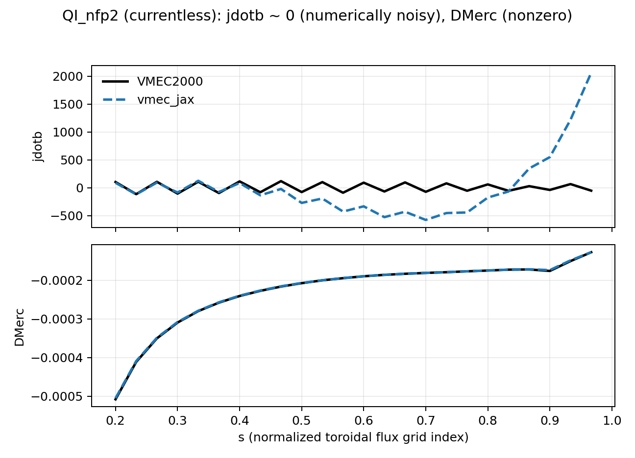
QI_nfp2 jdotb/DMerc parity (axis masked) — `QI_nfp2`: `jdotb` (cancellation-limited) and `DMerc` (nonzero).¶

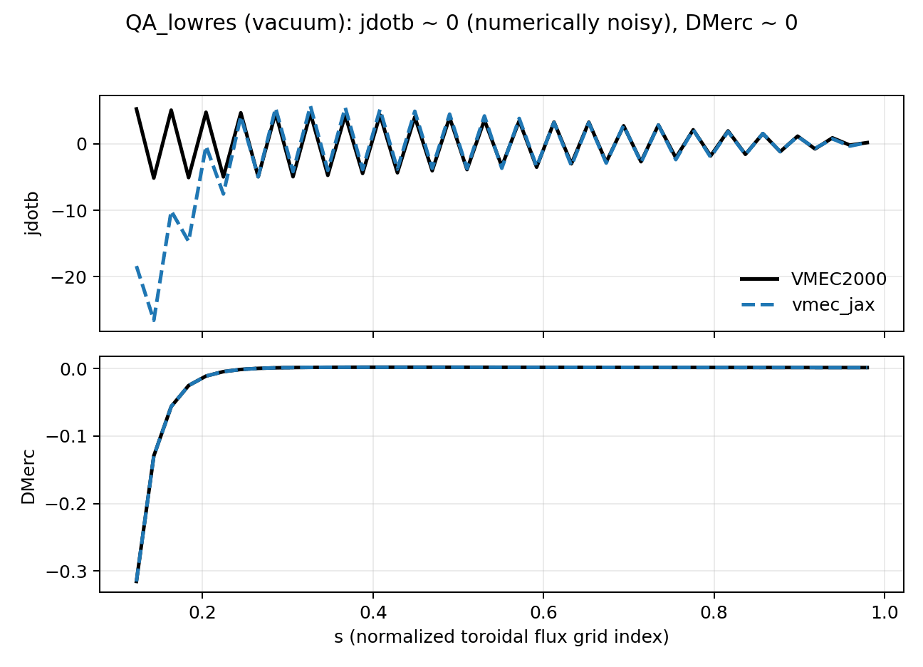
QA_lowres jdotb/DMerc parity (axis masked) — `LandremanPaul2021_QA_lowres`: vacuum-like case; `DMerc` should be ~0.¶

For current-driven cases, use the bundled reactor-scale QA/QH examples when a nonzero jdotb profile is needed for targeted parity checks. The small-signal QI/QA plots above remain the default documentation figures because they are the most stable examples for explaining the cancellation-limited behavior of jdotb and Mercier diagnostics.

Implementation Pointers (Source Code)¶

The relevant vmec_jax code paths are:

vmec_jax/wout.py:
- parity-channel construction for bsub{u,v},
- jxbforce-style low-pass filter and reconstruction,
- Mercier and jdotb assembly.

Performance Notes (vmec_jax vs VMEC2000)¶

VMEC2000 implements these diagnostics in Fortran with explicit loops over (m,n) modes and over the reduced (theta,zeta) grid. For parity work, vmec_jax originally mirrored this ordering closely, including Python-level loop nests for some cancellation-sensitive sums. That path is useful for debugging, but it is too slow to be a good default.

Today, vmec_jax uses vectorized NumPy contractions (einsum) for the wrout-style Nyquist analysis and the jxbforce filter by default. These vectorized paths preserve the VMEC2000 discretization but may change floating point summation order slightly.

If you need the slow loop order for debugging, the following env vars switch back to explicit loops:

VMEC_JAX_WROUT_LOOP=1: use loop-based wrout Nyquist analysis.
VMEC_JAX_JXBFORCE_LOOP=1: use loop-based jxbforce reconstruction of bsubsu/bsubsv.
VMEC_JAX_BSUB_FILTER_LOOP=1: use loop-based jxbforce low-pass filter.
VMEC_JAX_MERCIER_EXACT_SUM=1: use explicit theta/zeta summation order in Mercier surface averages.

The reference VMEC2000 implementations are:

bcovar.f (odd-channel storage convention for IEQUI=1 outputs)
jxbforce.f (filter and itheta/izeta/bdotk construction)
mercier.f (Mercier term assembly)

Reproducing The Figures¶

These figures were generated from VMEC-style wout_*.nc files using:

python tools/diagnostics/plot_wout_profiles_compare.py \
  --vmec /path/to/vmec2000/wout_case.nc \
  --jax  /path/to/vmec_jax/wout_case.nc \
  --vars jdotb,DMerc \
  --axis-skip 6 --drop-edge \
  --out docs/_static/figures/case_jdotb_dmerc_parity.png

JXBFORCE / Mercier Diagnostics (jdotb, DMerc)¶

Key VMEC2000 Convention: Parity Channels For bsubu/bsubv¶